Tutorial – Quantum dynamical effects in liquid water: A semiclassical study on the diffusion constant and the infrared absorption spectrum
TABLE OF CONTENTS
- 1. Introduction
- 2. Preparing topology and coordinate files
- 3. Classical Dynamics
- 4. Quantum Dynamics
- 5. Results and Discussion
- 6. Appendix
1. Introduction
This tutorial reproduces the calculations of the diffusion constant and IR spectrum of liquid water by employing path integral molecular dynamics (PIMD) and linearized semiclassical initial value representation (LSC-IVR) as described in the following paper:
It is designed for those who are going to run molecular dynamics simulations with quantum dynamic methods, PIMD and LSC-IVR. The prerequisites are listed as below:
AMBER 12 software package - sander and its parallel version, sander.MPI, are used to run dynamics simulations. In addition, LEaP (tleap and its graphical user interface, xleap) is utilized to generate the topology file of the water molecule and water box.
Packmol - Create the pdb file of water box, by packing single molecules in a defined region.
VMD - Visualize the structures and motions of molecules. It is optional here, but can be helpful to build the image of the model.
Note:
- The PIMD calculations in this tutorial require over 24 CPUs. Be sure you can afford such a job.
- One is supposed to know or can find the meanings of basic shell commands in Linux, such as
ls,pwd,cd,mkdir,cp,mv, and so on.- The shell scripts used in this tutorial are run in Linux platform, and should be set as executable first, then run in the terminal. For example, suppose one has a script file named ‘example.sh’, one may set it as executable by
chmod +x example.sh, then run in the terminal using the command./example.sh.
The tutorial is organized as follows: first we prepare topology and coordinate files for water model and minimize the energy. Then classical dynamics or quantum dynamics can be used to equilibrate and sample the system. We will show the two procedures separately. Finally, the results from classical dynamics and quantum dynamics are compared and discussed.
2. Preparing topology and coordinate files
In this section, we shall use LEaP and Packmol to create topology (prmtop) and coordinate (inpcrd) files for water box containing 216 water molecules.
2.1 Creating a pdb file for a single water molecule
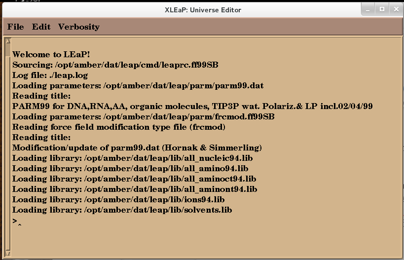
To begin with, we use the xleap tool to create a pdb file for a single water molecule. Start xleap with the following command:
$ xleap -s -f leaprc.ff99SBNote: the character '\$' denotes that this command is carried out in the terminal. Type the stuff after “\$”,then hit ‘Enter’.
The xleap window is now opened with the force field ‘FF99SB’ loaded, as shown in the figure below:
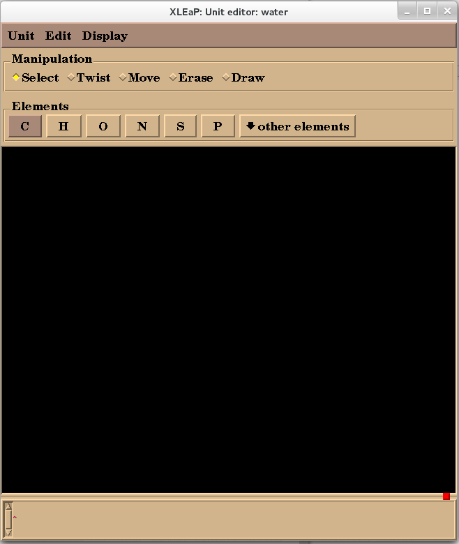
Then use the edit command to start an editor window named as ‘water’:
> edit waterNote: the character ‘>’ denotes that this command is carried out in the xleap window. Type the stuff after ‘>’, then hit ‘Enter’.
The editor window will look like this:
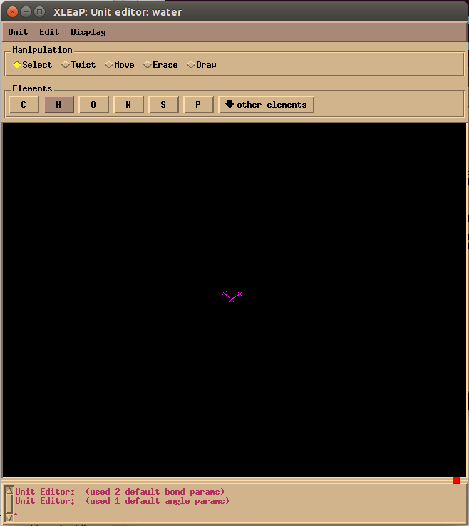
To draw the water molecule, first click on the O button in the Elements label and click on the black background to create an oxygen atom. Then click on H to draw two hydrogen atoms, then click on the oxygen and drag a line to each hydrogen to make ‘bond’. Afterwards, click the Select button in Manipulation label and double-click the background to select the whole molecule. At last, use Edit → Relax to ensure a right size of the water molecule. Remember to close the window by Unit → Close instead of X button at the corner, or you will exit xleap.
Note: you may turn off the Num/Caps lock to make the menu work.
Use the following command in xleap to save a pdb file for the water molecule:
> savepdb water water1.pdbUse File → Quit to close the xleap window. Then we have a pdb file named as ‘water1.pdb’. Here is an example:
   ATOM      1  O1  wat    1       0.770  -0.484   0.000  1.00  0.00
   ATOM      2  H2  wat    1       1.745  -0.706   0.000  1.00  0.00
   ATOM      3  H3  wat    1       0.235  -1.329   0.000  1.00  0.00
   TER
   END
The third and fourth columns should be changed manually to:
   ATOM      1  O   WAT    1       0.770  -0.484   0.000  1.00  0.00
   ATOM      2  H1  WAT    1       1.745  -0.706   0.000  1.00  0.00
   ATOM      3  H2  WAT    1       0.235  -1.329   0.000  1.00  0.00
   TER
   END
Otherwise, the water molecule will be treated as solvent instead of solute, or unrecognizable for AMBER package.
Note: the generated coordinates are probably different from the example, but the format should be consistent.
2.2 Creating a pdb file for a water box with 216 molecules
The Packmol program (you can download Packmol from http://www.ime.unicamp.br/~martinez/packmol/ and follow the installation instructions) is used to produce a file named ‘water216.pdb’ that describes 216 water molecules by inputting the file ‘water1.pdb’. The detailed steps are as follows:
1) Copy ‘water1.pdb’ file to the Packmol directory;
2) An input script named as ‘water.inp’ is required to be placed in the directory. Here is an example:
tolerance 2.0
output water216.pdb
filetype pdb
structure water1.pdb
number 216
inside cube 0. 0. 0. 19.
end structure| Settings | Summary |
|---|---|
| tolerance 2.0 | Defines the distance among the water molecules, with Angstrom (Å) as the unit. |
| output water216.pdb | Specifies the name of the output file, ‘water216.pdb’. |
| filetype pdb | Defines the format of output file. |
| structure water1.pdb | Declares the input structure file, ‘water1.pdb’. |
| number 216 | Specifies the number of water molecules |
| inside cube 0. 0. 0. 19. | Defines the size of the box: a cubic box with side length of 19 Å. |
The box length is estimated by
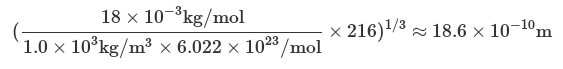
3) Run the script with the command:
$ ./packmol < water.inpThen a file ‘water216.pdb’ is created as follows:
 HEADER
 TITLE      Built with Packmol
 REMARK   Packmol generated pdb file
 REMARK   Home-Page: http://www.ime.unicamp.br/~martinez/packmol
 REMARK
 ATOM      1  O   WAT A   1      10.714   1.608  13.554  1.00  0.00
 ATOM      2  H1  WAT A   1      11.071   2.541  13.506  1.00  0.00
 ATOM      3  H2  WAT A   1      11.474   0.958  13.538  1.00  0.00
 ......
 ......
It should be mentioned that this pdb file cannot be used directly for the leap tool to create the prmtop and inpcrd files. To refine the pdb file generated by Packmol to be readable for AMBER, the following commands should be executed:
Call xleap with the force field ‘FF99SB’ loaded in the terminal:
$ xleap -s -f leaprc.ff99SBIn the xleap window, load and save pdb files by typing in following commands:
> wat216=loadpdb water216.pdb
> savepdb wat216 water216new.pdb
The structure is then loaded in LEaP and converted into a new pdb file named ‘water216new.pdb’, which will be used to setup the prmtop and inpcrd files for the water model in the following stages.
 ATOM      1  O   WAT     1      10.714   1.608  13.554  1.00  0.00
 ATOM      2  H1  WAT     1      11.071   2.541  13.506  1.00  0.00
 ATOM      3  H2  WAT     1      11.474   0.958  13.538  1.00  0.00
 TER
 ATOM      4  O   WAT     2      17.338   2.985  12.846  1.00  0.00
 ATOM      5  H1  WAT     2      17.363   2.369  12.058  1.00  0.00
 ATOM      6  H2  WAT     2      17.850   3.818  12.636  1.00  0.00
 TER
 ......
 ......
2.3 Imposing periodic boundary conditions and creating the topology and coordinate files
In this step, tleap is used to generate the inpcrd and prmtop files for further simulations. Here, a tleap script named ‘leaprc’ is written as follows:
source leaprc.protein.ff14SB
loadOff solvents.lib
WAT = SPG
loadAmberParams frcmod.qspcfw
set default FlexibleWater on
water = loadpdb "water216new.pdb"
setBox water centers 0.0
saveamberparm water wat216.prmtop wat216.inpcrd
quit
The script calls LEaP to load the AMBER parameters of the ‘q-SPC/Fw’ model, a water model including quantum effects. Then the pdb file of the water box is loaded and the center of box is set to 0.0. set default FlexibleWater on is used to avoid performing SHAKE to restraint bond lengths. Finally, the AMBER parameters, together with the topology information, and coordinates from the pdb file are saved to the prmtop and inpcrd files, respectively.
Run the script with tleap:
$ tleap leaprcThen the prmtop and inpcrd files are generated. Take a look at the ‘wat216.inpcrd’ file:
 default_name
 648
 10.5626559   1.7106296  12.9585540  10.9196559   2.6436296  12.9105540
 11.3226559   1.0606296  12.9425540  17.1866559   3.0876296  12.2505540
 ......
 ......
 14.2776559  11.9276296  10.9425540  13.1276559   2.0116296   6.5545540
 13.4336559   1.1126296   6.2375540  12.2416559   2.2266296   6.1465540
 19.0010000  19.0000000  19.0000000  90.0000000  90.0000000  90.0000000
The first line gives the name of this inpcrd file, which was not defined and is default here. The second line specifies the number of atoms in this system, and the following data are the coordinates of each atom. The last line defines the cubic box with a size of 19.0 Å *19.0 Å *19.0 Å , which remains to be further optimized in the following sections.
Note: the generated box size will be probably not exactly 19.0 Å, but should be close.
The ‘wat216.prmtop’ file gives the parameter and topology information of the system, such as atomic number, atom type, charges, bonding and non-bonded interactions, etc. For more details of the prmtop file, please visit http://ambermd.org/formats.html#topology.
%VERSION  VERSION_STAMP = V0001.000  DATE = 06/04/14  16:08:11
%FLAG TITLE
%FORMAT(20a4)
default_name
%FLAG POINTERS
%FORMAT(10I8)
     648       2     648       0     216       0       0       0       0       0
     864     216       0       0       0       2       1       0       2       1
       0       0       0       0       0       0       0       1       3       0
       0
%FLAG ATOM_NAME
%FORMAT(20a4)
O   H1  H2  O   H1  H2  O   H1  H2  O   H1  H2  O   H1  H2  O   H1  H2  O   H1
... ... ...
H1  H2  O   H1  H2  O   H1  H2
%FLAG CHARGE
%FORMAT(5E16.8)
 -1.53067320E+01  7.65336600E+00  7.65336600E+00 -1.53067320E+01  7.65336600E+00
  7.65336600E+00 -1.53067320E+01  7.65336600E+00  7.65336600E+00 -1.53067320E+01
... ... ...
2.4 Minimizing the energy of the system
It is necessary to run minimization to optimize the coordinates of the water box. The input file ‘min.in’ that includes the settings for minimization is as follows:
 minimization
 &cntrl
 imin   = 1,
 maxcyc = 50000,
 ncyc   = 25000,
 ntb    = 1,
 cut    = 7.0
/| Settings | Summary |
|---|---|
| imin=1 | Do minimization |
| maxcyc=50000 | Specify the number of maximum cycles for minimization |
| ncyc=25000 | Use the steepest descent algorithm for the first 0-ncyc cycles, then switch to the conjugate gradient algorithm for ncyc-maxcyc cycles |
| ntb=1 | Periodic boundary conditions are employed, with constant volume |
| cut=7.0 | Non-bonded cutoff distance in Angstroms |
Run the minimization with sander:
$ sander -O -i min.in -p wat216.prmtop -c wat216.inpcrd -o min.out -r min.rstAfter minimization, two files, ‘min.out’ and ‘min.rst’, are obtained.
The ‘min.out’ file contains information of energy, bond length, angle, and so on. The script process_minout.perl in $AMBERHOME/AmberTools/bin/ can be used to analyse the output.
$ process_minout.perl min.outThe energy must be converged after minimization. Otherwise, you need to increase the numbers maxcyc and ncyc and redo the minimization.
The restrt file ‘min.rst’ includes the information of coordinates which will be used for the following stage. Here is an example of ‘min.rst’ file.
default
648
11.7654710   1.3373752  13.0319944  11.6694818   2.0964767  12.3503829
11.7890772   0.4629812  12.4992566  16.0994647   3.2814888  11.4881731
16.2442149   2.2743210  11.3714834  16.2335751   3.4755383  12.4814771
...
...
16.6067259  10.5627386   9.8208016  16.4186102  11.5458786   9.9309056
16.3603299  10.1591423  10.7382855  12.0189548   1.7739896   6.4213408
12.8127279   1.1745325   6.1790117  11.9893955   2.5238504   5.7258450
19.0040000  19.0280000  19.0180000  90.0000000  90.0000000  90.0000000
Till now, the topology and coordinate files, ‘wat216.prmtop’ and ‘min.rst’ respectively, have been prepared. They will be used to start classical dynamics and quantum dynamics simulations in the following stages.
3. Classical Dynamics
The flowchart for classical dynamics is as follows:

In this section, we use classical molecular dynamics to calculate the diffusion constant and IR spectrum of 216 water molecules. The simulations are performed in a cubic box with the periodic boundary conditions. We run an NPT simulation first to obtain the density for liquid water under the condition of 298.15 K and 1 atm, and then an NVT simulation to obtain canonical equilibrium properties. After equilibrating the system, we sample the coordinates and velocities from the NVT ensemble, which will be used as the initial conditions for classical trajectories in the NVE ensemble. We have analyzed our results and shown them at the end of section.
NVE: constant number (N), volume (V), and energy (E); the sum of kinetic (KE) and potential energy (PE) is conserved, temperature (T) and pressure (P) are unregulated.
NVT: constant number (N), volume (V), and temperature (T); T is regulated via a thermostat; P is unregulated.
NPT: constant number (N), temperature (T) and pressure (P); T is regulated via a thermostat and P is regulated via a bariostat; V is unregulated.
3.1 Equilibrating the system using classical dynamics (NPT)
The ‘min.rst’ file obtained from minimization is used as the inpcrd file, together with the prmtop file ‘wat216.prmtop’ to run an NPT simulation. In this stage, the NPT simulation is carried out for 4.0 ns to obtain convergent density. The whole simulation can be separated into 8 steps. The input files (‘npt1.in’ and ‘npt2.in’) are as follows:
NPT simulation of liquid water
&cntrl
imin = 0,
irest = 0, ntx = 1,
ntb = 2, cut = 7.0,
ntp = 1,taup = 4.0, pres0 = 1.013, barostat = 1,
tempi = 298.15, temp0 = 298.15,
ntt = 3, gamma_ln = 5.0, ig = -1,
nstlim = 1000000, dt = 0.0005,
ntpr = 50, ntwx = 1000, ntwr = 1000
/
&ewald
skinnb = 2.0
/
NPT simulation of liquid water
&cntrl
imin = 0,
irest = 1, ntx = 5,
ntb = 2, cut = 7.0,
ntp = 1,taup = 4.0, pres0 = 1.013, barostat = 1,
tempi = 298.15, temp0 = 298.15,
ntt = 3, gamma_ln = 5.0, ig = -1,
nstlim = 1000000, dt = 0.0005,
ntpr = 50, ntwx = 1000, ntwr = 1000
/
&ewald
skinnb = 2.0
 /
| Settings | Summary |
|---|---|
| imin = 0 | Do not do minimization |
| irest = 0 | Do not restart the simulation |
| ntx = 1 | Only read coordinates from input |
| irest = 1 | Restart the simulation |
| ntx = 5 | Read both the coordinates and velocities from input |
| ntb = 2 | Constant pressure periodic boundary conditions are used |
| cut = 7.0 | Non-bonded cutoff distance in Angstroms |
| ntp = 1 | With isotropic position scaling |
| taup = 4.0 | Pressure relaxation time (in ps), recommended value is between 1.0 and 5.0, default is 1.0. |
| pres0 = 1.013 | Reference pressure (in bar) at which the system is to be kept |
| barostat = 1 | Use Berendsen barostat |
| tempi = 298.15 | Initial temperature (in K) |
| temp0 = 298.15 | Reference temperature (in K) at which the system is to be kept |
| ntt = 3 | Langevin thermostat is used |
| gamma_ln = 5.0 | Collision frequency (in ps-1) for Langevin dynamics |
| ig = -1 | Random seed is initialized with current date and time. |
| nstlim = 1000000 | Number of steps to be performed |
| dt = 0.0005 | The size of time step (in ps) |
| ntpr = 50 | Energy information will be written to mdout and mdinfo every 10 steps |
| ntwx = 1000 | The coordinates will be written to the mdcrd file every 10 steps |
| ntwr = 1000 | The restrt file will be written every 10 steps during dynamics |
| skinnb=2.0 | Width of the nonbonded “skin” (in Å), default is 2.0 Å. The direct sum nonbonded list is extended to cut+skinnb |
We note that the periodic boundary conditions involve truncation of interactions. In Amber 12, there are two parameters relative to truncation of interaction, cut and skinnb. Use of skinnb is required for energy conservation, and the value 2.0 (Å) is recommended for all particle mesh Ewald (PME) runs. The direct sum non-bonded list is extended to cut + skinnb, and the van der Waals and direct electrostatic interactions are truncated at cut. A larger cutoff introduces less error in the non-bonded force evaluation but increases the computational complexity and thus calculation time. You need to choose a value for the non-bonded cutoff for this liquid water system. Note that when the periodic boundary condition is on, the largest value of cutoff should be less than half the side length of the periodic box. Here, this value should be 9.0 Å (7.0 Å for cut and 2.0 Å for skinnb).
We use Langevin dynamics as the thermostatting method, with the collision frequency given by gamma_ln (in ps-1). Note that it is not necessary that gamma_ln approximates the physical collision frequency, which is about 50 ps-1 for liquid water. It is often advantageous to use much smaller value around 2 to 5 ps-1. The ig option determines the random seed. When ig is set as -1, the random seed is initialized with current date and time.
One can run the NPT simulation with the shell script below:
#!/bin/bash
sander -O -i npt1.in -p wat216.prmtop -c min.rst  -o npt.out.1 -r npt.rst.1 -x mdcrd1
sander -O -i npt2.in -p wat216.prmtop -c npt.rst.1 -o npt.out.2 -r npt.rst.2 -x mdcrd2
sander -O -i npt2.in -p wat216.prmtop -c npt.rst.2 -o npt.out.3 -r npt.rst.3 -x mdcrd3
sander -O -i npt2.in -p wat216.prmtop -c npt.rst.3 -o npt.out.4 -r npt.rst.4 -x mdcrd4
sander -O -i npt2.in -p wat216.prmtop -c npt.rst.4 -o npt.out.5 -r npt.rst.5 -x mdcrd5
sander -O -i npt2.in -p wat216.prmtop -c npt.rst.5 -o npt.out.6 -r npt.rst.6 -x mdcrd6
sander -O -i npt2.in -p wat216.prmtop -c npt.rst.6 -o npt.out.7 -r npt.rst.7 -x mdcrd7
sander -O -i npt2.in -p wat216.prmtop -c npt.rst.7 -o npt.out.8 -r npt.rst.8 -x mdcrd8
Here, ‘min.rst’, ‘npt1.in’, ‘npt2.in’ and ‘wat216.prmtop’ are the input files, while the files ‘npt.out.*’, ‘npt.rst.*’ and ‘mdcrd*’ (* represents 1-6) are the results of the NPT simulation.
Note that the size of the box indicated in ‘npt.rst.1’ is no longer 19.0Å*19.0Å*19.0Å, but 18.52Å*18.54Å*18.53Å or something around this. We can summary the results and analyze the distribution by using some tools provided by Amber. For example, use the process_mdout.perl script (You can find it in $AMBERHOME/AmberTools/bin/) as follows:
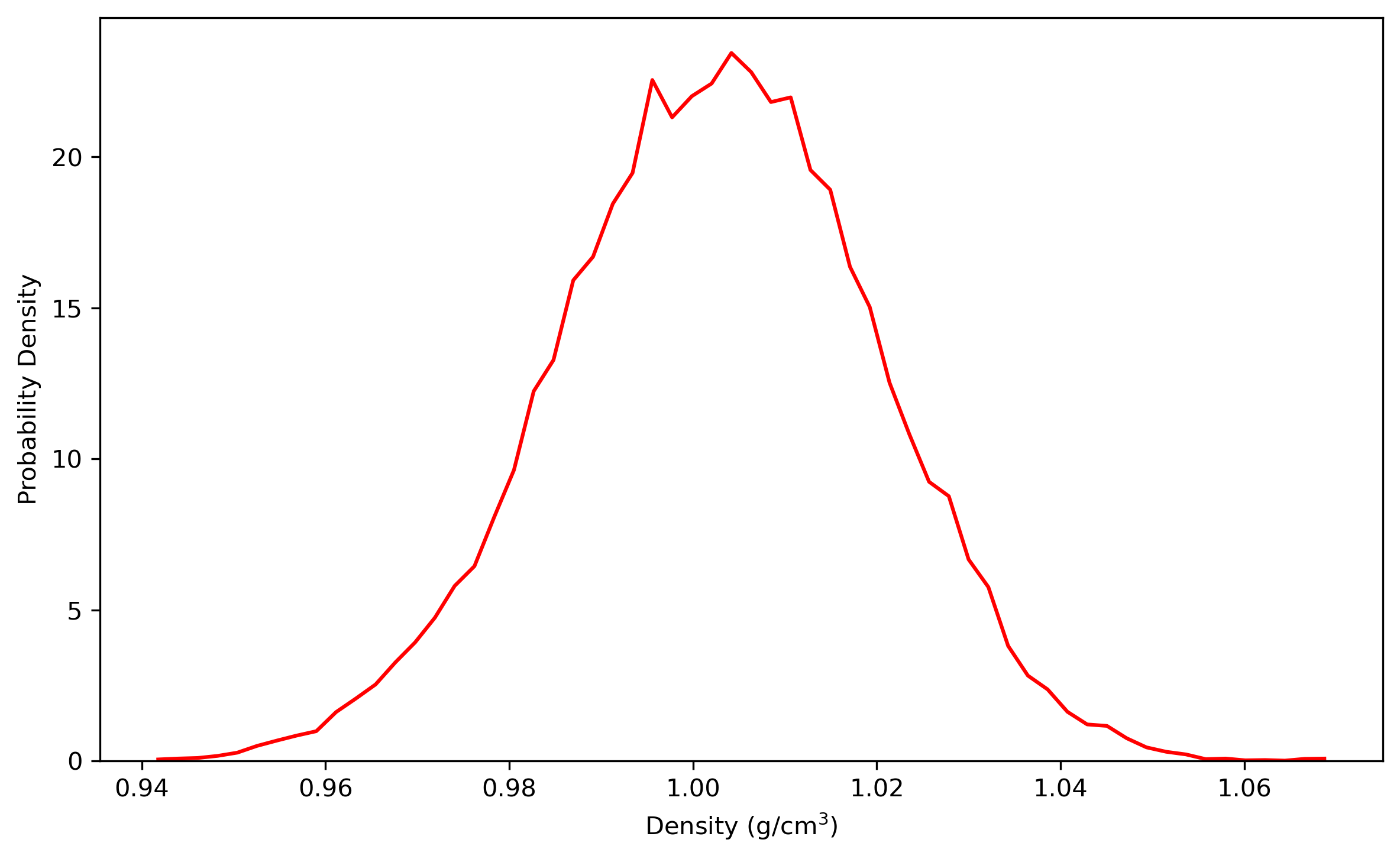
$ process_mdout.perl npt.out.3 npt.out.4 npt.out.5 npt.out.6 npt.out.7 npt.out.8Then we have a series of summary files. Use python to plot the results:
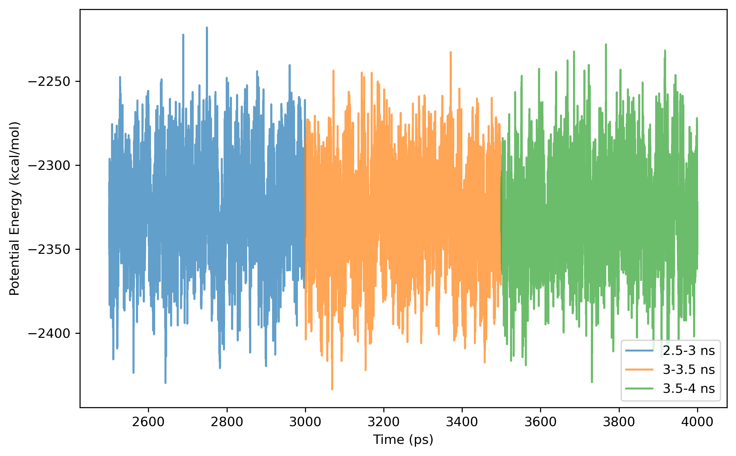
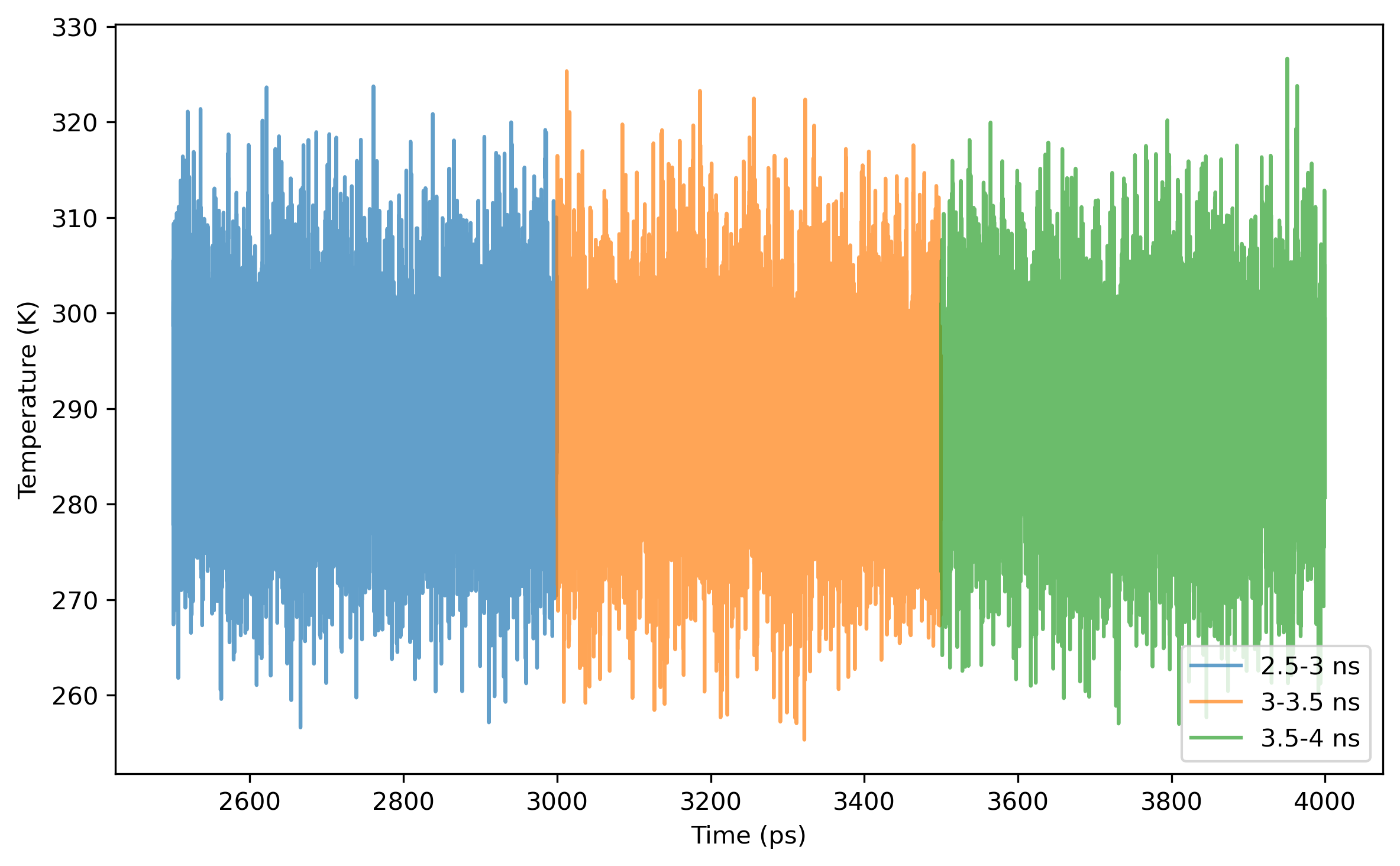
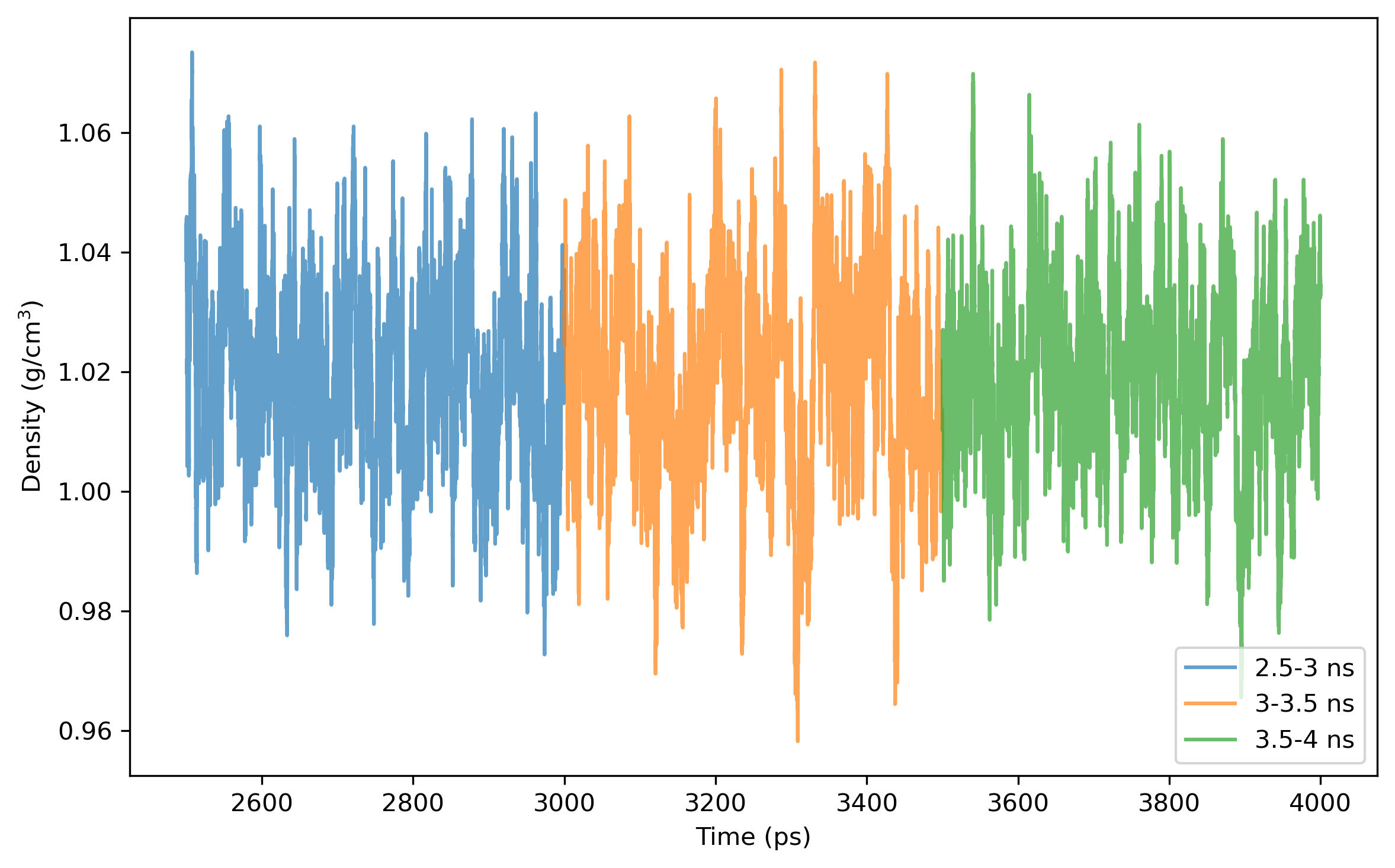
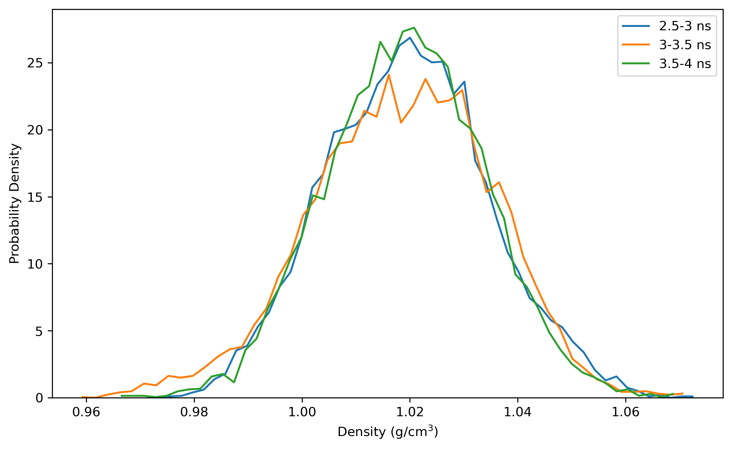
Note: the density of the last time step should be around the average value, otherwise it is not a good point to start NVT simulation.
3.2 Equilibrating the system using classical dynamics (NVT)
In the previous stage, we have obtained a convergent density about 1.018 g/ml, for the liquid water system. In this stage, an NVT simulation will be carried out for a targeted temperature, 298.15 K. The whole simulation of 1.6 ns, will be separated into 8 steps. The input file is as follows:
NVT simulation of liquid water
&cntrl
imin = 0,
irest = 1, ntx = 5,
ntb = 1, cut = 7.0,
ntt = 3, gamma_ln = 5.0, ig = -1,
tempi = 298.15, temp0 = 298.15,
nstlim = 400000, dt = 0.0005,
ntpr = 10, ntwr = 10, ntwv = 10, ntwx = 10
/
&ewald
skinnb = 2.0
/
In this mdin file, most settings are similar to the NPT simulation, except ntb=1, which means periodic boundaries are imposed on the system with constant volume. The option ntp=0 is default for no pressure scaling and not required to written here.
Run the NVT simulation with the following Shell script:
#!/bin/bash
sander -O -i nvt.in -p wat216.prmtop -c npt.rst.6  -o nvt.out.1 -r nvt.rst.1 -x mdcrd7
sander -O -i nvt.in -p wat216.prmtop -c nvt.rst.1 -o nvt.out.2 -r nvt.rst.2 -x mdcrd8
sander -O -i nvt.in -p wat216.prmtop -c nvt.rst.2 -o nvt.out.3 -r nvt.rst.3 -x mdcrd9
sander -O -i nvt.in -p wat216.prmtop -c nvt.rst.3 -o nvt.out.4 -r nvt.rst.4 -x mdcrd10
sander -O -i nvt.in -p wat216.prmtop -c nvt.rst.4 -o nvt.out.5 -r nvt.rst.5 -x mdcrd11
sander -O -i nvt.in -p wat216.prmtop -c nvt.rst.5 -o nvt.out.6 -r nvt.rst.6 -x mdcrd12
sander -O -i nvt.in -p wat216.prmtop -c nvt.rst.6 -o nvt.out.7 -r nvt.rst.7 -x mdcrd13
sander -O -i nvt.in -p wat216.prmtop -c nvt.rst.7 -o nvt.out.8 -r nvt.rst.8 -x mdcrd14
Here ‘npt.rst.6’, ‘nvt.in’, ‘wat216.prmtop’ are the input files. After the simulation is done, use the following command to obtain the summary files:
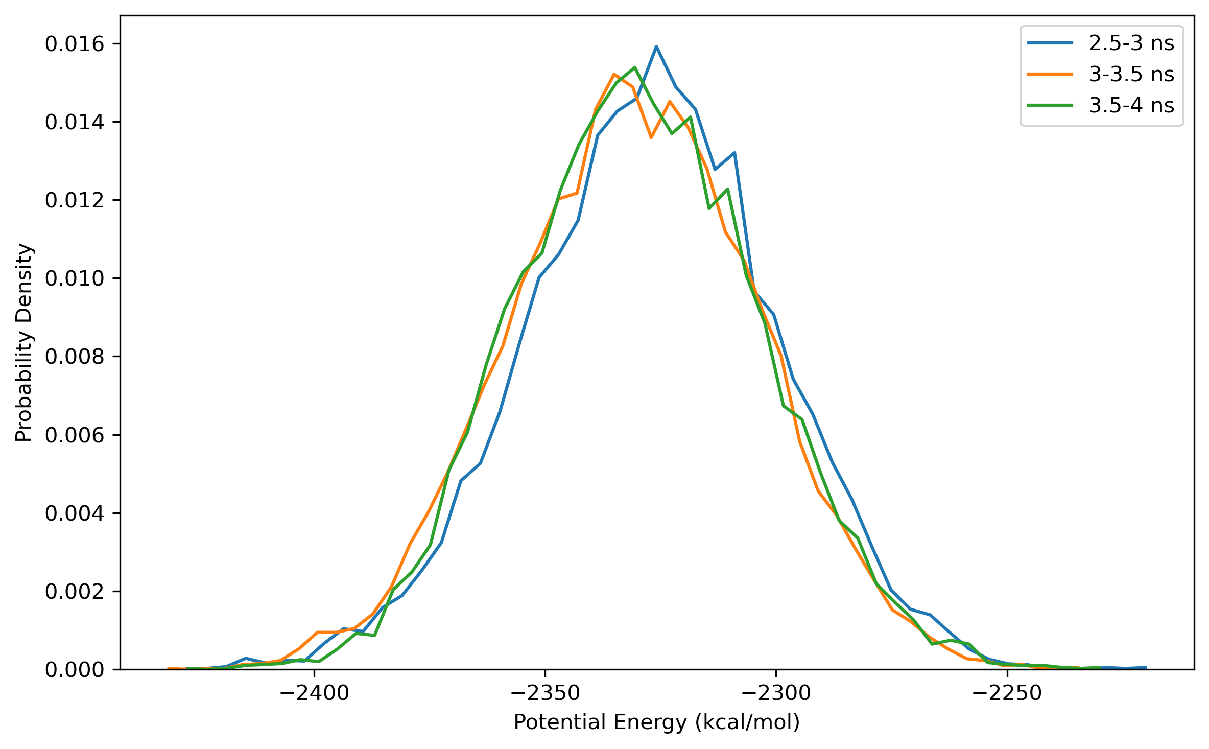
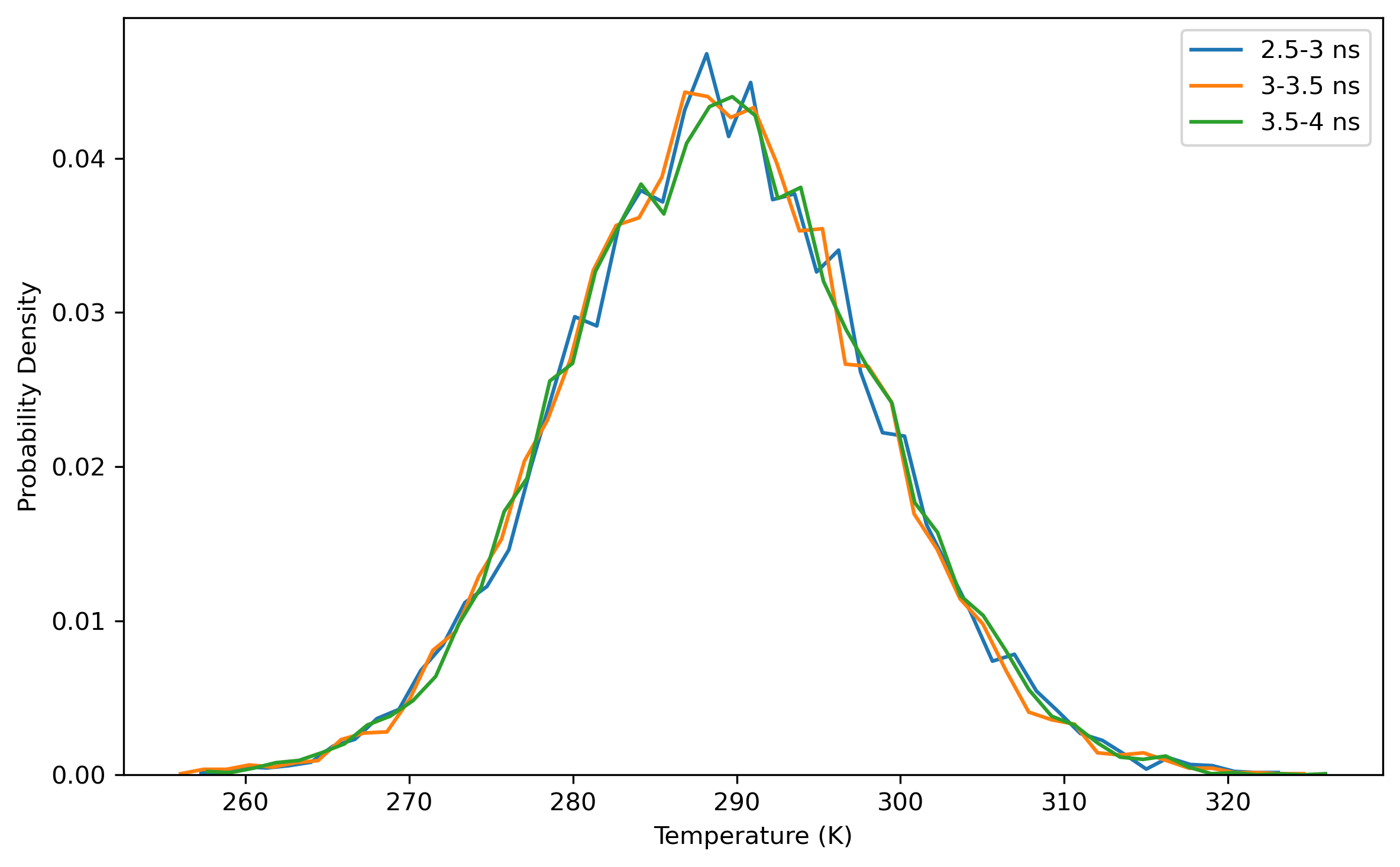
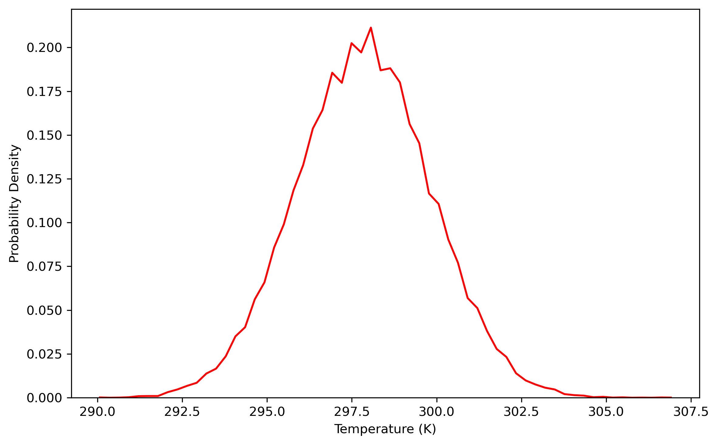
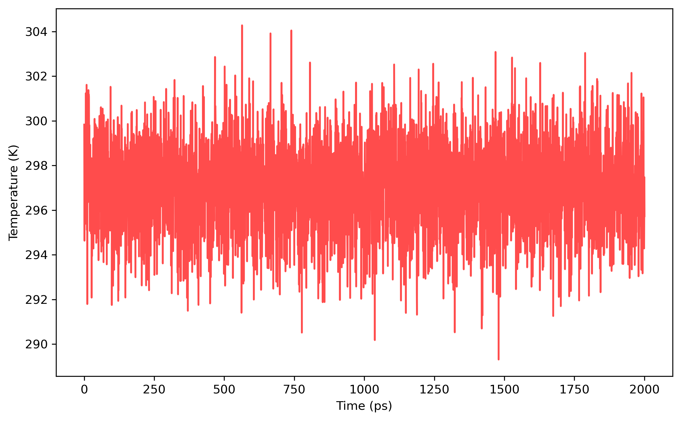
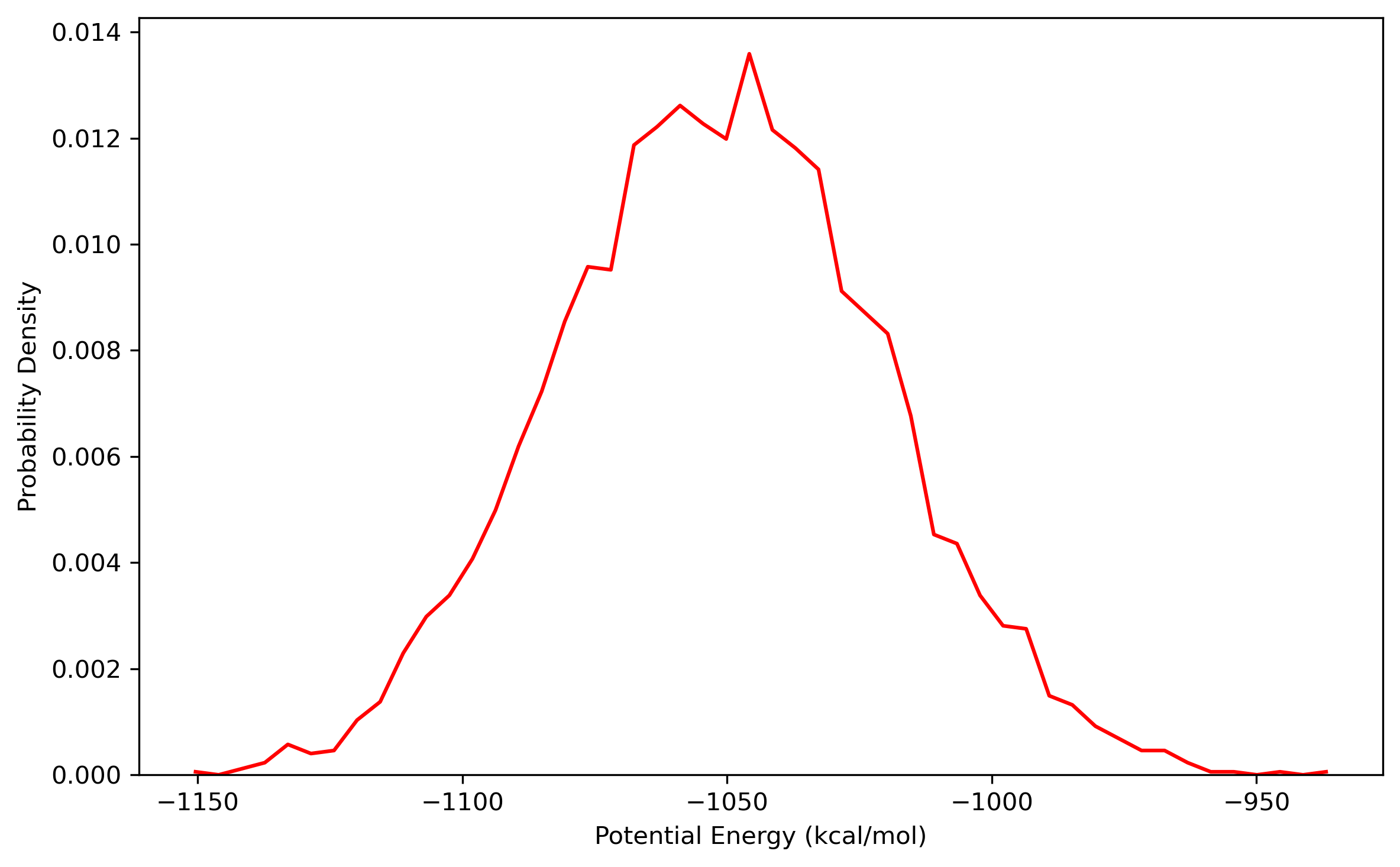
$ process_mdout.perl nvt.out.1 nvt.out.2 nvt.out.3 nvt.out.4 nvt.out.5 nvt.out.6 nvt.out.7 nvt.out.8Then you may use python to obtain the distribution diagrams of potential energy and temperature:


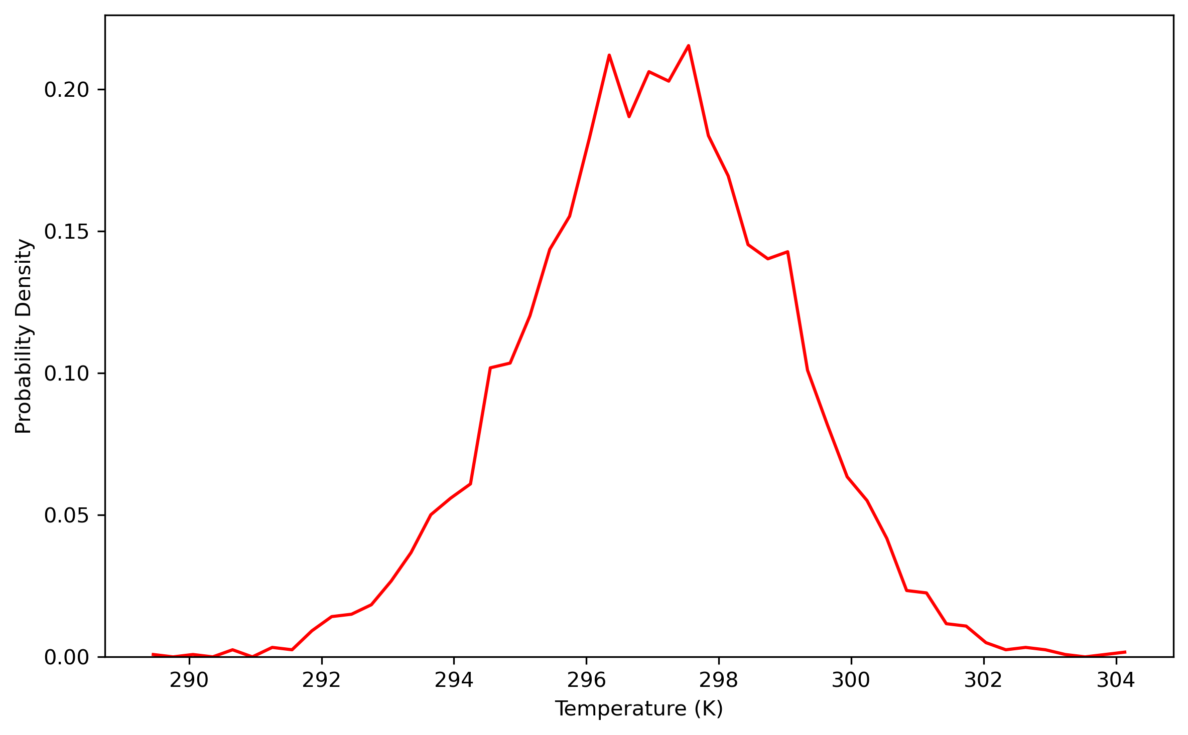
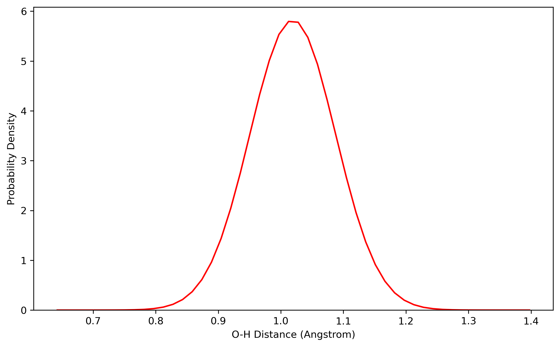
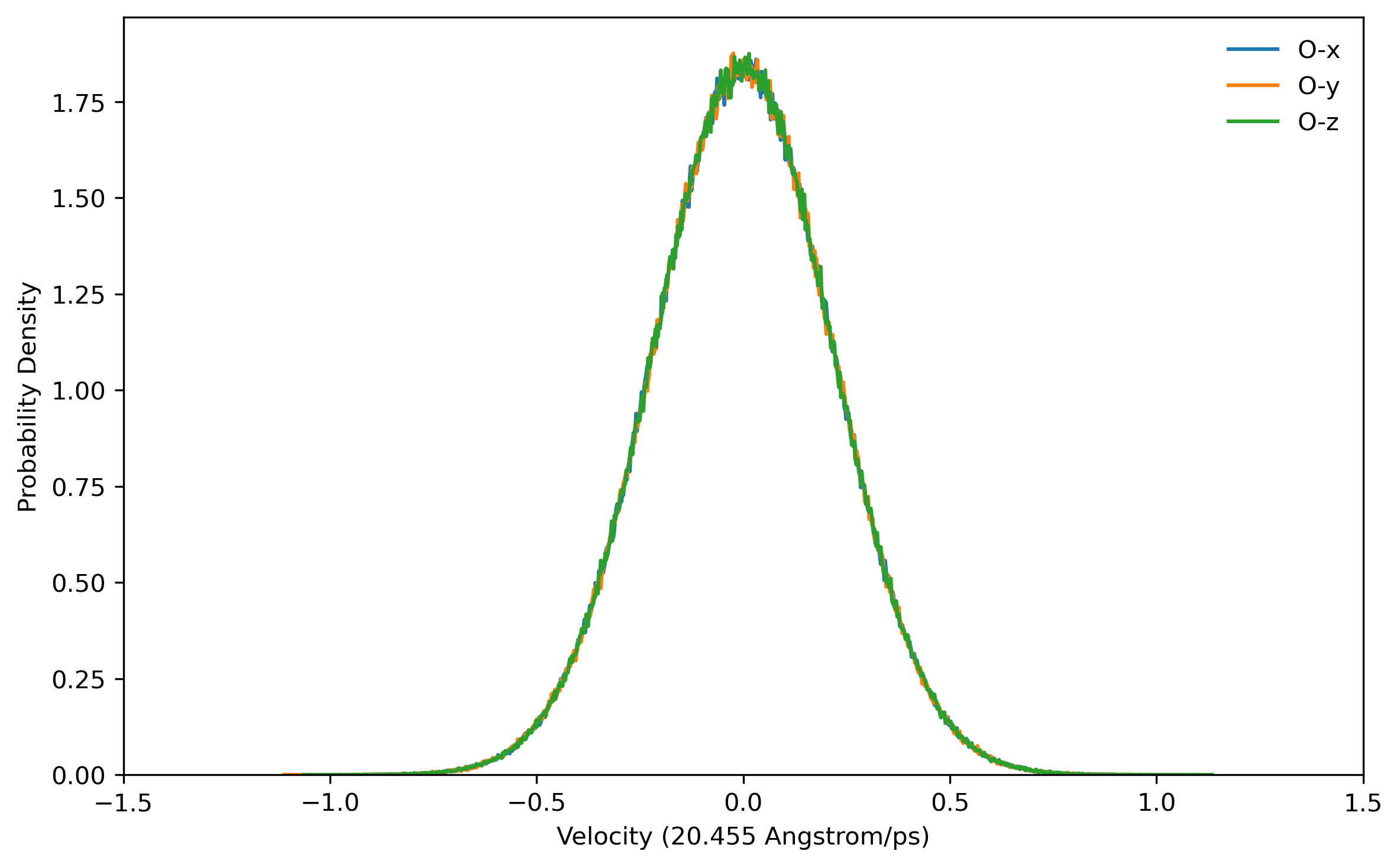
Also, the distribution of coordinates and velocities during this step is shown below:


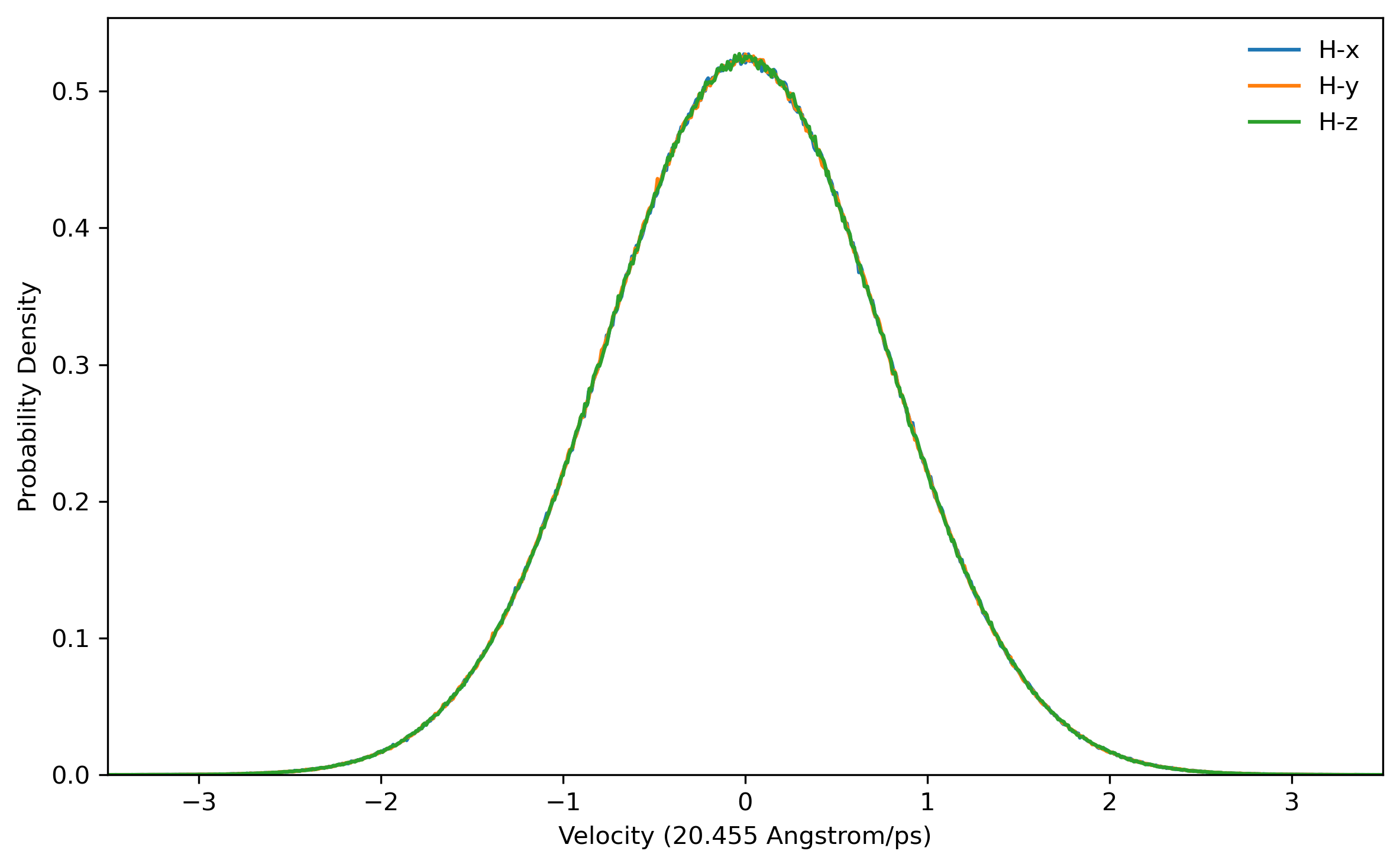
Fig. 3.3. Distribution of coordinates and velocities of water molecule over a 1.6 ns simulation
3.3 Sampling from the NVT ensemble
Now the system of 216 water molecules is in canonical equilibrium. Initial coordinates and velocities will be sampled in the NVT ensemble for the following NVE simulation. The time interval for the sampling will be 2 ps. Correlation functions from classical dynamics will be both time-averaged and trajectory-averaged. In this tutorial, 100 samples are produced with the restrt file 'nvt.rst.4' in the previous step. The samples are then used to gain good statistics for the correlation functions.
For convenience, a loop script is used for sampling:
#!/bin/bash
for (( i=1; i<=100; i++ )); do
    echo $i
    sander -O -i sample.in -c nvt.rst.4 -p wat216.prmtop -r sample.rst -o sample.out
    mkdir $i
    cp sample.rst $i/
    mv sample.rst nvt.rst.4
done
and the input file is shown below, which indicates that we take the sampling for every 2 ps.
Classical MD sample
&cntrl
imin = 0,
irest = 1, ntx = 5,
ntb = 1, cut = 7.0
ntt = 3, gamma_ln = 5.0, ig = -1,
tempi = 298.15, temp0 = 298.15
nstlim = 4000, dt = 0.0005,
ntpr = 10, ntwr = 10, ntwv = 10, ntwx = 10
/
&ewald
skinnb = 2.0
/
After executing the loop script, we then have 100 folders named from 1 to 100, each with an restrt file ‘sample.rst’ inside.
3.4 Propagating classical trajectories in the NVE ensemble
In this step, we use the samples obtained from the previous NVT simulation to carry out NVE simulations to propagate classical trajectories. A loop script is used here:
#!/bin/bash
for (( i=1; i<=100; i++ )); do
    echo $i
    cp nve.in wat216.prmtop $i
    cd $i
    sander -O -i nve.in -c sample.rst -p wat216.prmtop -r nve.rst -o nve.out
    cd ..
done
The coordinates and velocities contained in the sample, i.e. ‘sample.rst’ in each folder, are used as initial conditions of each trajectory. The input file is as follows:
NVE simulation of liquid water
&cntrl
imin = 0,
irest = 1, ntx = 5,
ntt = 0, cut = 7.0,
ntb = 1,
nstlim = 40000, dt = 0.0005,
nscm = 1,
ntpr = 1, ntwr = 1, ntwx = 1, ntwv = 1
/
&ewald
skinnb = 2.0
/
The parameter nscm is set as a flag for the removal of translational and rotational center-of-mass (COM) motion at regular intervals (default is 1000). Here we do the removal at each step.
The input files are: nve.in, nve.sh, wat216.prmtop.
3.5 Analysis
The velocities in each mdvel file of the corresponding trajectory are used to calculate the center-of-mass velocity autocorrelation function and the dipole-derivative autocorrelation function required for diffusion constant and IR spectrum calculation.
3.5.1 Diffusion constant
The self-diffusion constant of a single water molecule can be obtained from the center-of-mass velocity autocorrelation function:
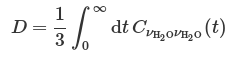
The center-of-mass velocity of single water molecule can be obtained from the center-of-mass momentum, which is the sum of the momenta of the two hydrogen atoms and that of the oxygen atom.
Fortran code com-vacf.f90 is used to calculate center-of-mass velocity autocorrelation function. The parameters in the code e.g. nstep, dt etc. may be modified according to your own settings.

3.5.2 Infrared spectrum
The experimental IR spectrum is given in terms of two frequency-dependent properties, the Beer-Lambert absorption constant α(ω) and the refractive index n(ω). These quantities are related to the Fourier transform of the dipole-derivative autocorrelation function:
The fortran code duacf.f90 is used to calculate dipole-derivative autocorrelation function:

The parameters in the code e.g. nstep, dt etc. may be modified according to your own settings.
The infrared intensities is obtained from the Fourier transform of dipole-derivative autocorrelation function. The results are plotted below:
4. Quantum Dynamics
After preparation of the liquid water model and energy minimization, quantum dynamics methods are used to study the diffusion constant and infrared spectrum in this section. The results are then compared with those from classical dynamics.
The flowchart for quantum dynamics is as follows:
4.1 Equilibrating the system with PIMD (NPT)
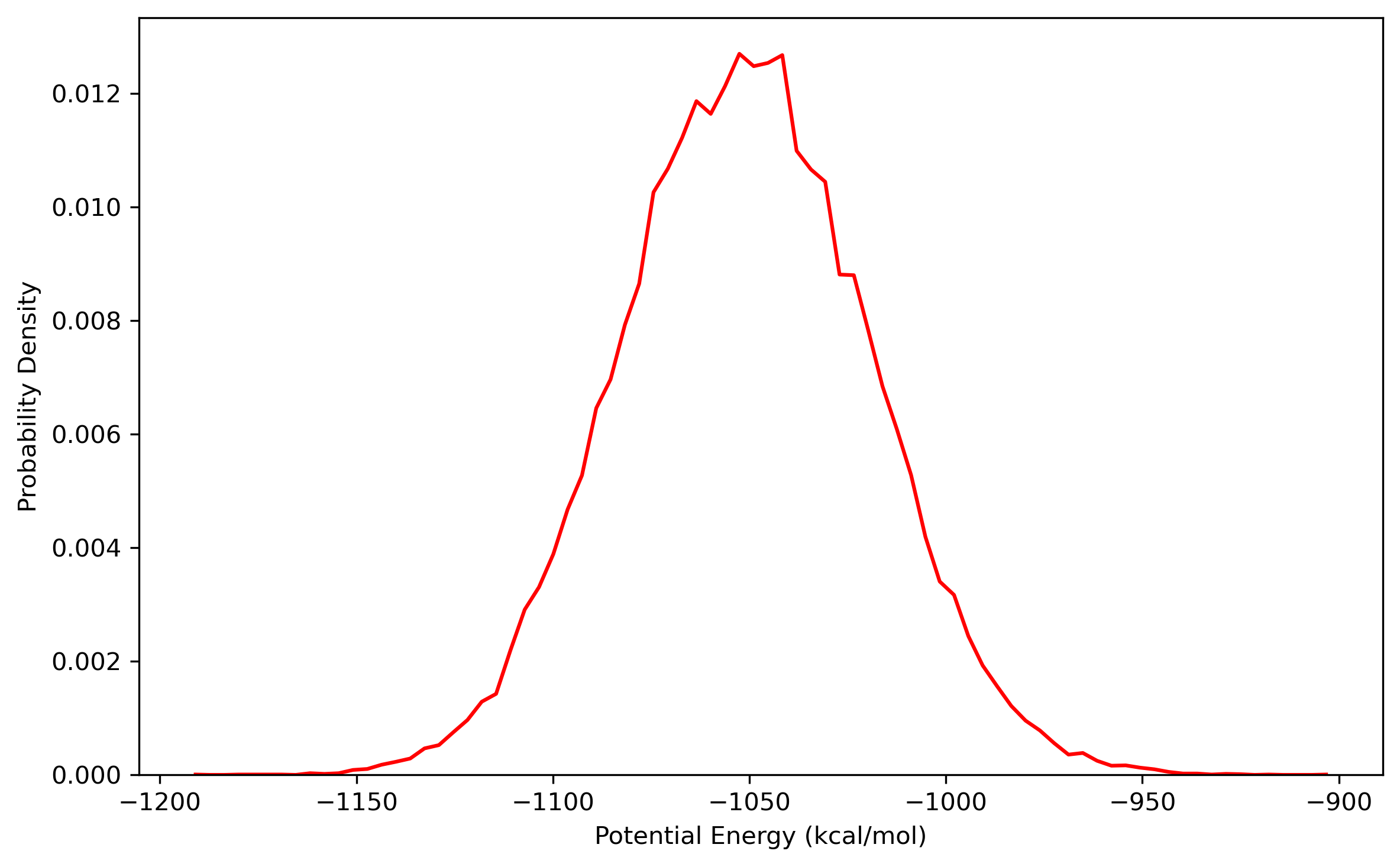
The PIMD NPT simulation is required for the density of the system. Before simulation, one may estimate the size of time step (dt) from the vibration period of a ring polymer (Tp), which can be deduced from the equation below:
A reasonable estimate for the size of time step is dt = Tp/300, e.g. about 0.1 fs for 24 beads at 298.15 K. The number of beads should be tested and chosen carefully for convergence of results.
To run the PIMD NPT simulation, parallel version of Amber program with sander.MPI exploiting the multisander scheme is used.
An example of the command is as follows:
$ mpirun -np 24 sander.MPI -ng 24 -groupfile gf_npt_pimd1With this command, the job will be run using sander.MPI with 24 CPU cores which are separated into 24 groups, and the groups file ‘gf_npt_pimd1’ contains the options for sander.MPI, which might be like this:
-O -i pimd_npt1.in -p wat216.prmtop -c min.rst -r npt1.rst
-O -i pimd_npt1.in -p wat216.prmtop -c min.rst -r npt2.rst
... ... ...
-O -i pimd_npt1.in -p wat216.prmtop -c min.rst -r npt24.rst
A simple shell script can be used to generate this groups file with a loop:
#!/bin/bash
# write gf_npt_pimd
n=24
for (( i=1; i<=$n; i++ )); do
    echo "-O -i pimd_npt1.in -p wat216.prmtop -c min.rst -r npt${i}.rst"
done > gf_npt_pimd1
The mdin, prmtop and inpcrd files are essential for the computation. The prmtop file is the same as the one used in classical dynamics simulation which is generated from model preparation. The inpcrd file is ‘min.rst’, obtained from energy minimization, which is also the same as the one initially used in classical dynamics simulation. The mdin file (‘pimd_npt1.in’) which contains settings for PIMD NPT is given below, together with the mdin file which reads both coordinates and velocities from previous restrt file.
NPT simulation of liquid water
 &cntrl
 ipimd = 2
 irest = 0, ntx = 1
 ntb = 2, cut = 7.0, ntp = 1
 pres0 = 1.013, taup=4.0,
 tempi = 298.15, temp0 = 298.15
 ntt = 4, nchain = 4, gamma_ln = 2
 nscm = 1000
 nstlim = 2000000, dt = 0.0001
 ntpr = 1000, ntwx = 1000, ntwr = 1000
  /
 &ewald
 skinnb = 2.0
 /
NPT simulation of liquid water
&cntrl
ipimd = 2
irest = 1, ntx = 5
ntb = 2, cut = 7.0, ntp = 1
pres0 = 1.013, taup=4.0,
tempi = 298.15, temp0 = 298.15
ntt = 4, nchain = 4, gamma_ln = 2
nscm = 1000
nstlim = 2000000, dt = 0.0001
ntpr = 1000, ntwx = 1000, ntwr = 1000
 /
&ewald
skinnb = 2.0
/
| Settings | Summary |
|---|---|
| ipimd=2 | Normal Mode Path Integral Molecular Dynamics (NMPIMD) is used |
| irest=0 | Do not restart the simulation |
| ntx=1 | Only read coordinates from input |
| irest=1 | Restart the simulation |
| ntx=5 | Read both the coordinates and velocities from input |
| ntb=2 | Constant pressure periodic boundary conditions are used |
| ntp=1 | with isotropic position scaling |
| cut=7.0 | Non-bonded cutoff distance in Angstroms |
| tempi=298.15 | Initial temperature (in K) |
| temp0=298.15 | Reference temperature (in K) at which the system is to be kept |
| ntt=4 | Constant temperature, use Nosé-Hoover chain method for thermostats |
| nchain=4 | Number of thermostats in each Nosé-Hoover chain of thermostats (default 2, recommended >= 4) |
| taup=4.0 | Pressure relaxation time (in ps), recommended value is between 1.0 and 5.0, default is 1.0. |
| pres0=1.013 | Reference pressure (in bar) at which the system is to be kept |
| nscm=1000 | Remove translational and rotational center-of-mass motions every 1000 steps, default |
| nstlim=2000000 | Number of steps to be performed |
| dt=0.0001 | The size of time step (in ps) |
| ntpr=1000 | Energy information will be written to mdout and mdinfo every 1000 steps |
| ntwx=1000 | The coordinates will be written to the mdcrd file every 1000 steps |
| ntwr=1000 | The restrt file will be written every 10 steps during dynamics |
| skinnb=2.0 | Width of the nonbonded “skin” (in Å), default is 2.0 Å. The direct sum nonbonded list is extended to cut+skinnb |
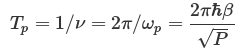
As the job runs, pimdout file which reports the quantum results for the whole system (i.e. total, kinetic and potential energy, pressure, volume, density, etc.) will be generated. Because Nosé-Hoover chains of thermostats are employed, an additional file ‘NHC.dat’ is written with the conserved energy for the extended system. The simulation may be time-consuming to achieve convergence, therefore it is necessary to separate the simulation into several steps, and run them sequently. For the first step only the coordinates are read and the velocities are generated, so irest=0 and ntx=1 are used. For the following steps, both the coordinates and velocities are read from the restrt files generated by the previous step, so irest=1 and ntx=5 are used, and the mdin file and groups file should be modified respectively. When each job finishes, the results shall be checked carefully.
Here is an example script to run the whole job:
#!/bin/bash
# run 1 step using min.rst as coordinate file in the groups file (gf_npt_pimd1),
# and then 4 steps using the generated restrt files (npt*.rst) as coordinate files in the groups file (gf_npt_pimd2)

nc=24
# write gf_npt_pimd1
for (( i=1; i<=${nc}; i++ )); do
    echo "-O -i pimd_npt1.in -p wat216.prmtop -c min.rst -r npt${i}.rst"
done > gf_npt_pimd1

# run the first step
mpirun -np ${nc} sander.MPI -ng ${nc} -groupfile gf_npt_pimd1
for (( i=1; i<=${nc}; i++ )); do
    cp npt${i}.rst npt${i}.rst.0 # backup the restrt files
done
cp pimdout pimdout.0 # backup pimdout file

# write gf_npt_pimd2
for (( i=1; i<=${nc}; i++ )); do
    echo "-O -i pimd_npt2.in -p wat216.prmtop -c npt${i}.rst -r npt${i}.rst.new"
done > gf_npt_pimd2

nstep=4
for (( j=1; j<=${nstep}; j++ )); do
    # each run is a restart from previous step
    mpirun -np ${nc} sander.MPI -ng ${nc} -groupfile gf_npt_pimd2
    for (( i=1; i<=${nc}; i++ )); do
        cp npt${i}.rst.new npt${i}.rst.${j} # backup the restrt files
        mv npt${i}.rst.new npt${i}.rst # prepare the restrt files for next run
    done
    cp pimdout pimdout.${j}  # backup pimdout file
done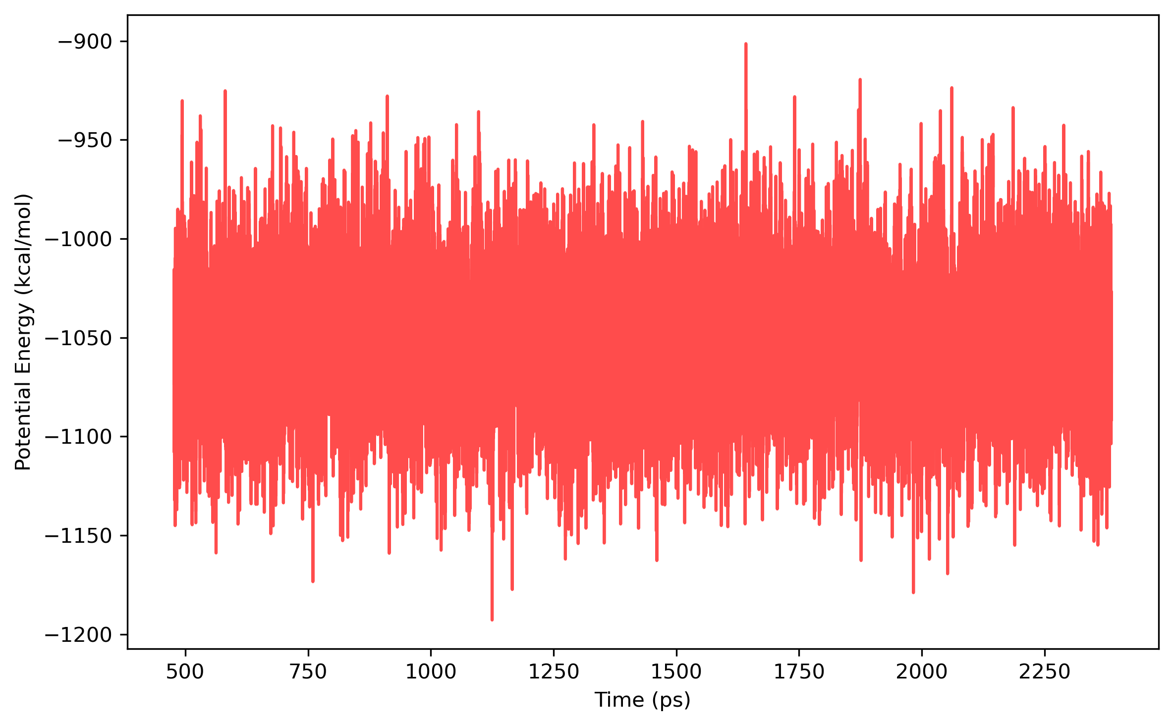

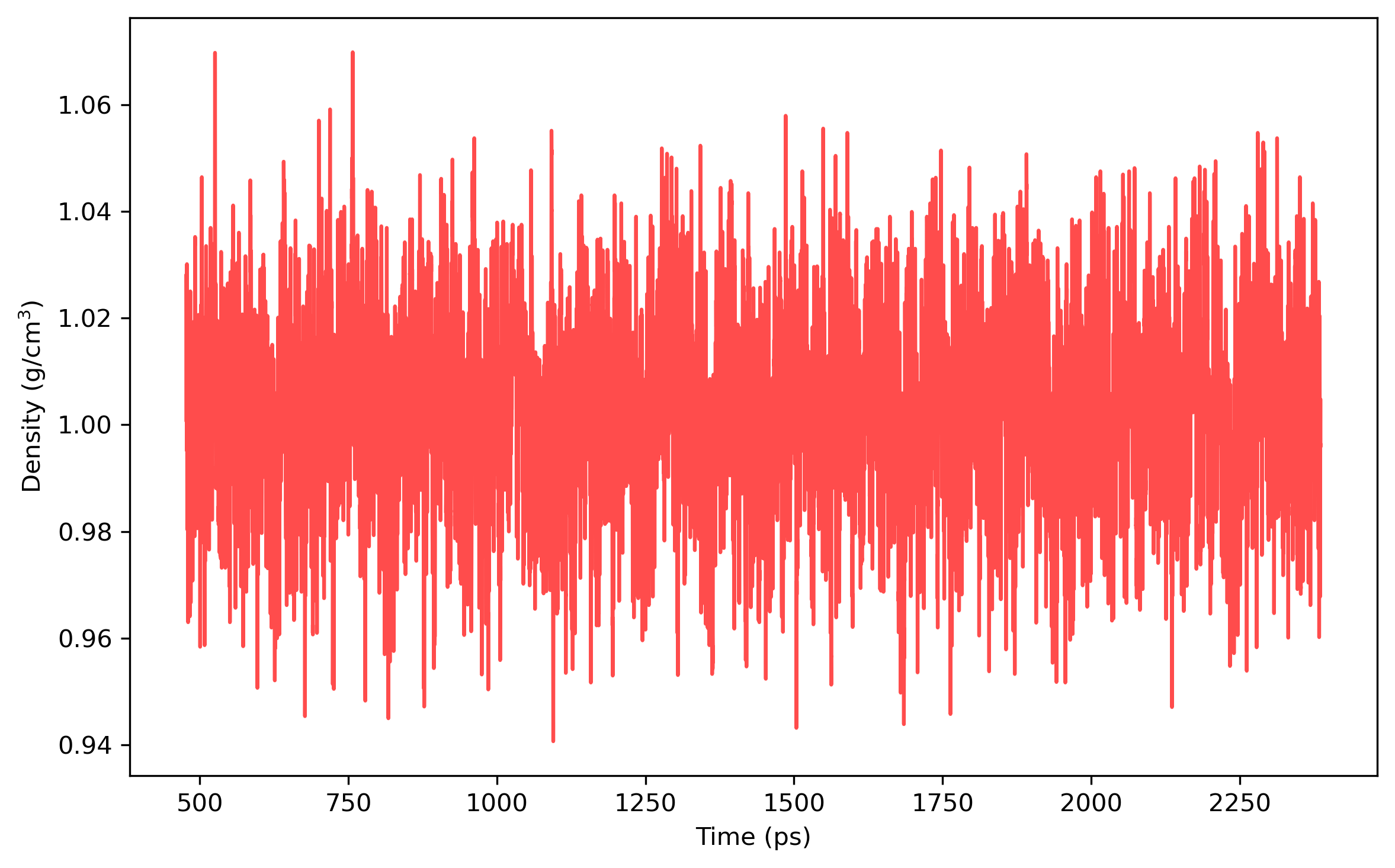
Once the density is converged, it is time to start PIMD simulation in the NVT ensemble in the next stage. The average density should be around the value of 1.002 g/ml.
Note: the density of the last time step should be around the average value, otherwise it is not a good point to start NVT simulation.
4.2 Equilibrating the system with PIMD (NVT)
In this stage, a long-time PIMD job (separated to several steps) is carried out in the NVT ensemble for the equilibrium of the system. The simulation is carried out with sander.MPI using the following command:
$ mpirun -n 24 sander.MPI -ng 24 -groupfile gf_nvt_pimdThe corresponding groups file ‘gf_nvt_pimd’ is like this:
 -O -i pimd_nvt.in -p wat216.prmtop -c npt1.rst -r nvt1.rst
 -O -i pimd_nvt.in -p wat216.prmtop -c npt2.rst -r nvt2.rst
......
 -O -i pimd_nvt.in -p wat216.prmtop -c npt24.rst -r nvt24.rst
Here the options are similar to the ones of PIMD simulation in the NPT ensemble. The restrt files produced from the previous step (‘npt*.rst’, * denotes 1-24) are used as the initial coordinates and velocities. 24 restrt files named as ‘nvt*.rst’ (here * denotes 1-24) are produced during the simulation. The energy information are written in the pimdout file.
pimd nvt
 &cntrl
  ipimd = 2
  ntb = 1,cut = 7.0,
  temp0  = 298.15, tempi = 298.15,
  ntt = 4, nchain = 4,
  dt = 0.0001, nstlim = 2000000,
  nscm = 1000,
  ntx = 5, irest = 1,
  ntwx = 1000,
  ntwr = 1000,
  ntpr = 1000,
 /
 &ewald
  skinnb = 2.0
 /
The PIMD simulation in the NVT ensemble is carried out for 2 ns. Here a script pimd_nvt.sh is used to do the job, which is similar to the one used in previous PIMD NPT simulation. The mdin file 'pimd_nvt.in' is the same in each step. The restrt files are used as inpcrd files for the next step.
The convergence of results shall be checked in the way as what is done in the PIMD NPT simulation. The distribution of the coordinates generated from the PIMD NVT simulation should satisfy Gaussian distribution.
For example, the results are plotted as follows:

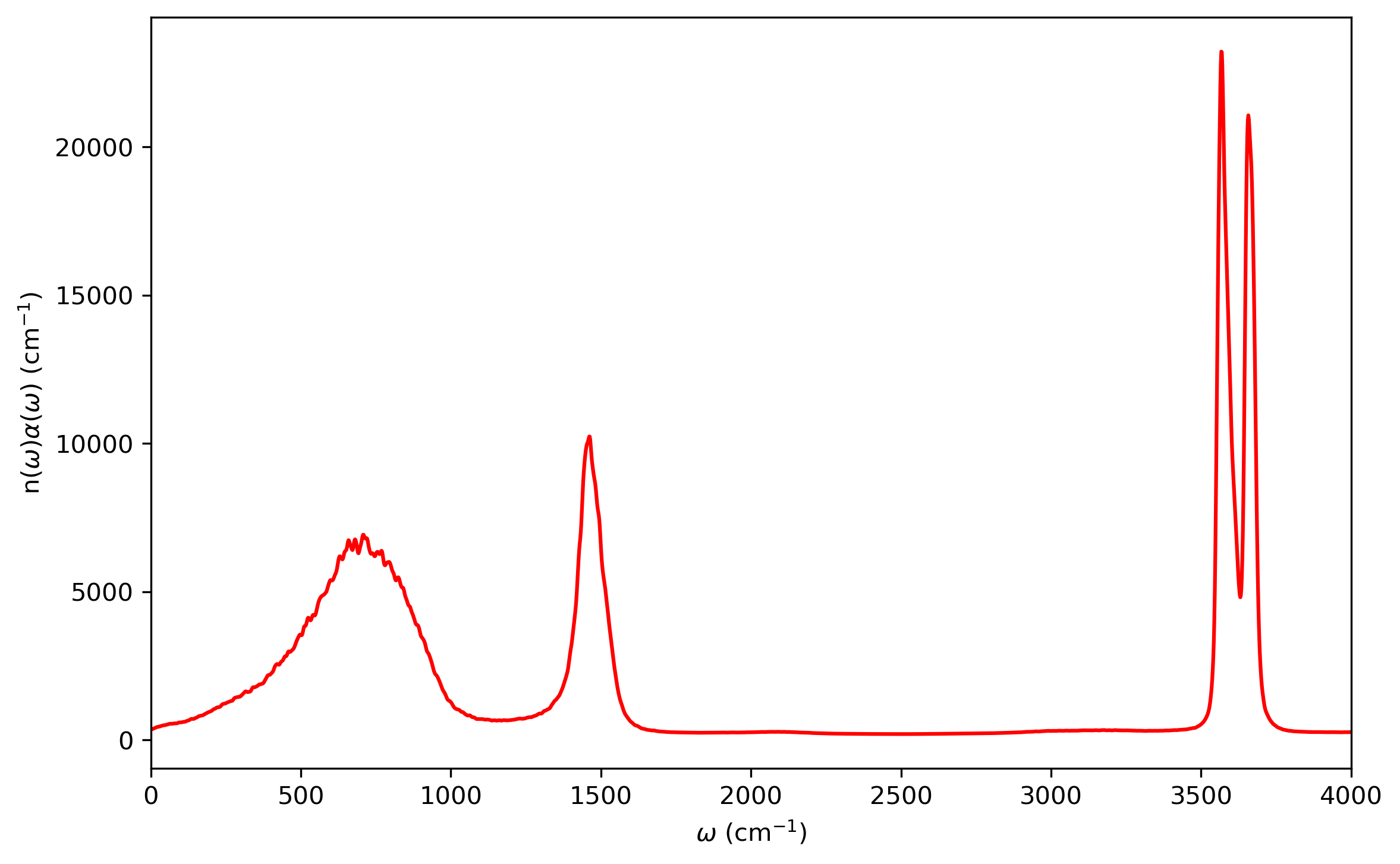
4.3 Sampling with PIMD (NVT)
After the equilibrium is achieved, sampling of coordinates from the NVT ensemble with PIMD is required for LSC-IVR simulation. This can be done by continuing the equilibrating process step by step, each for, e.g. 1 ps, The restrt files generated from the previous step are used as the inpcrd file for the next step, and more importantly, saved for further use as the inpcrd file for the LSC-IVR calculation, i.e., the ‘sample’. In this tutorial, 8000 steps are conducted to collect enough samples, with restrt files from each step saved in a different directory.
The following shell script is used to do this job:
#!/bin/bash
nsamp=8000
nc=24
for (( i=1; i<=${nsamp}; ++i ))
do
    mkdir ${i} # make work dir
    mpirun -n ${nc} sander.MPI -ng ${nc} -groupfile gf_sample # run pimd
    for (( j=1; j<=${nc}; ++j ))
    do
        cp nvt${j}.rst.new ${i}/        # copy generated coordinate files to work dir
        mv nvt${j}.rst.new nvt${j}.rst  # for next run
    done
done-O -i pimd-sample.in -c nvt1.rst -p wat216.prmtop -r nvt1.rst.new -o nvt1.out
-O -i pimd-sample.in -c nvt2.rst -p wat216.prmtop -r nvt2.rst.new -o nvt2.out
... ... ...
-O -i pimd-sample.in -c nvt24.rst -p wat216.prmtop -r nvt24.rst.new -o nvt24.outsample from NVT
&cntrl
ipimd = 2
ntb = 1,cut = 7.0,
temp0 = 298.15, tempi = 298.15,
ntt = 4, nchain = 4,
dt = 0.0001, nstlim = 10000,
nscm = 1000,
ntx = 5, irest = 1,
ntwx = 10,
ntwr = 10,
ntpr = 10,
/
&ewald
skinnb = 2.0
/The samples should be checked for the distribution of coordinates, which should resemble a Gaussian distribution.
4.4 LSC-IVR calculations
After the sampling is done, linearized semiclassical initial value representation (LSC-IVR) method is used to propagate real time trajectories from which the quantum thermal correlation functions can be obtained. The initial coordinates are randomly selected from the 24 restrt files generated in the previous step. Initial velocities are generated from the 0th step of LSC-IVR using LGA.
The example of mdin file for LSC-IVR is as follows:
LSC-IVR
 &cntrl
 ilscivr = 1, icorf_lsc = 4,
 ntx = 1, irest = 0,
 ntb = 1, cut = 7.0,
 ntt = 0,  temp0 = 298.15
 nscm = 1,
 dt = 0.0002, nstlim = 10000

 ntpr = 1, ntwx = 1, ntwv = 1
 /
 &ewald
 skinnb=2.0
/| Settings | Summary |
|---|---|
| ilscivr = 1 | Use LSC-IVR |
| icorf_lsc = 4 | Kubo-transformed correlation functions. This option affects output files for LSC-IVR only. |
Note: besides mdin, inpcrd and prmtop files, LSC-IVR requires a file named ‘LSC_rhoa.dat’ with an arbitary integer number between 0 and 10000 in it, which is used to generate the initial random number for the LSC-IVR calculation. As the number of trajectories for LSC-IVR is increased, it will automatically be updated.
A bash script can be used to run the LSC-IVR calculation for all the samples.
#!/bin/bash
# do LSC-IVR in each sample directory
nsamp=8000 # number of samples
nc=24
for (( i=1; i<=${nsamp}; ++i ))
do
cp lsc.in wat216.prmtop ${i} # copy essential files into work dir
cd ${i} # enter work dir
echo "$i" > LSC_rhoa.dat # preparation for LSC-IVR, here i should in the range between 0 and 10000
samp=$(( RANDOM%${nc} + 1 )) # randomly select sample as initial configuration
cp nvt${samp}.rst.new sample.rst
echo ${samp} > selected_sample # record selected sample for debug
echo "LSC-IVR for sample $i"
sander -O -i lsc.in -p wat216.prmtop -c sample.rst -r lsc.rst -o lsc.out
cd .. # exit work dir, back to parent dir
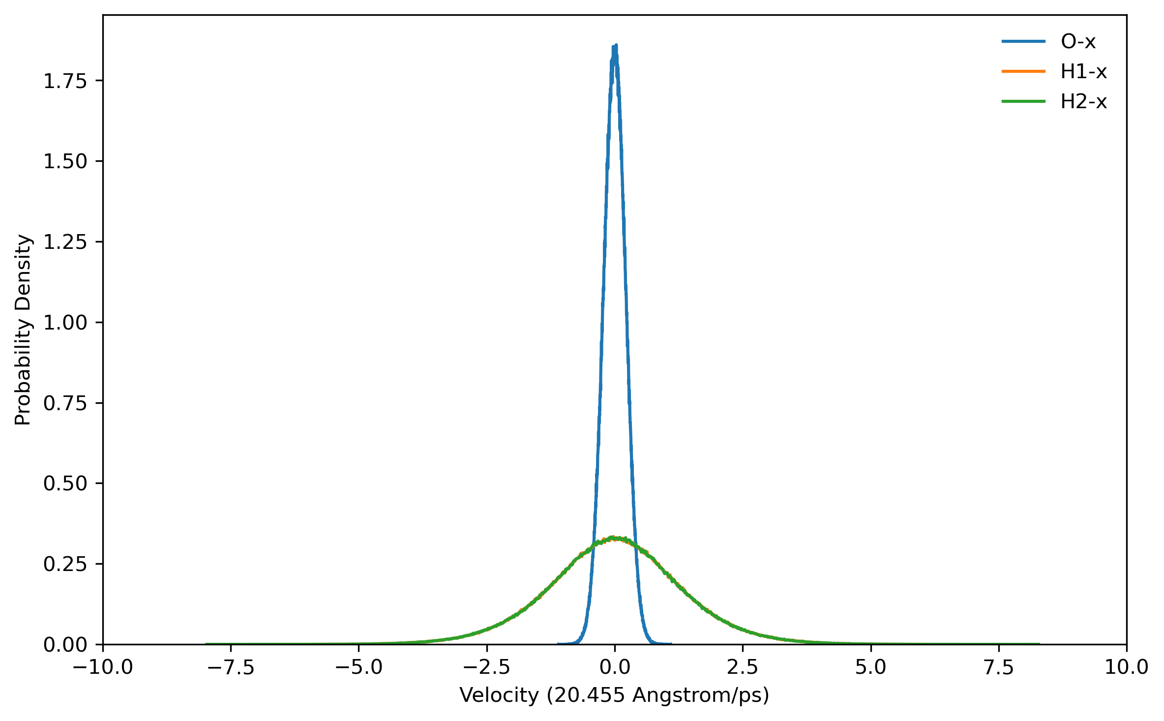
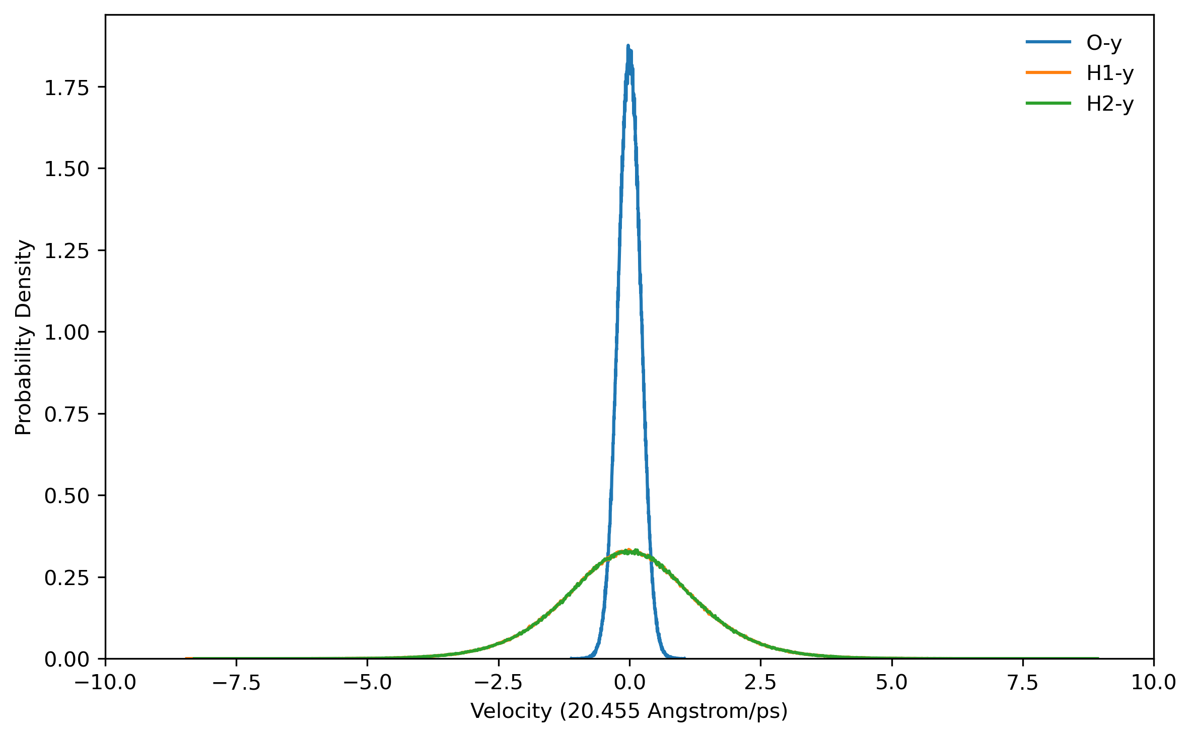
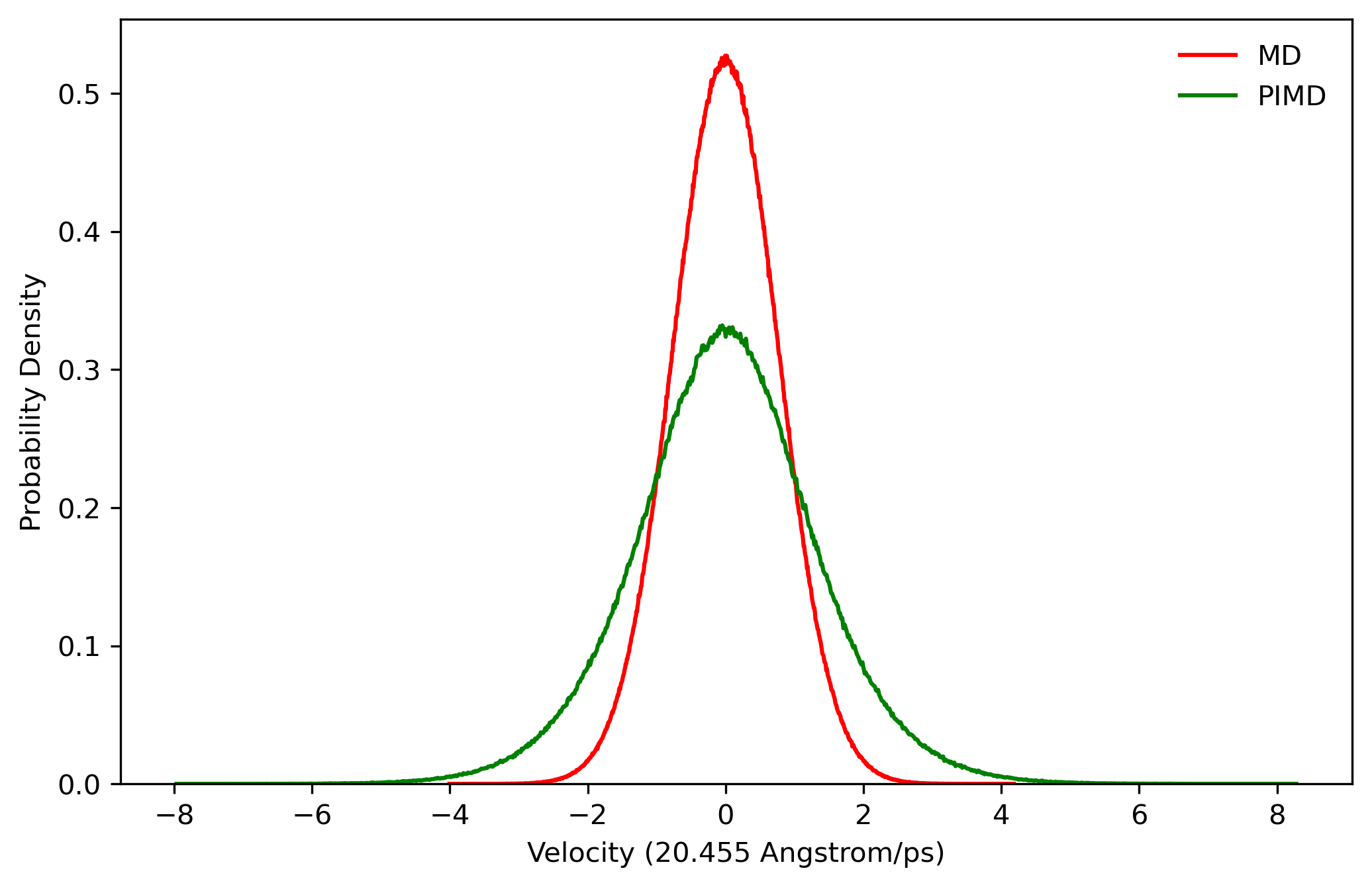
doneBefore running a long time job, it is necessary to test the settings are right. This can be done by running a job with only the initialization of LSC-IVR by setting nstlim=0 in ‘lsc.in’. One can find the generated initial velocities in the ‘LSC_rhoa.dat’ file in each sample directory. The velocity distributions of oxygen and hydrogen atom should be Gaussian distribution. Example results are plotted below:


Note: The generated trajectory files mdvel and mdcrd usually occupy disk space of hundreds of MB per sample. To save space, it is recommended to calculate the correlation functions cumulatively, and remove the used trajectories after correlation function calculation.
4.5 Analysis
To analyze the trajectories (mdvel and mdcrd files) propagated from the LSC-IVR calculations, a fortran code lsc_cor.f90 is written to summarize the results and calculate the correlation functions required for the diffusion constant and IR spectrum cumulatively. The parameters nstep and dtstep in ‘lsc_cor.f90’ should be modified to your own settings. A directory ‘lsc’ is built to place the results. In the parent directory, one can find that ‘lsc’ is parallel to the sample directories ‘1’, ‘2’, and so on using the ls command.
Before running the executable from compilation of ‘lsc_cor.f90’, a file named as ‘LSC_cor-216-vv.dat’ with the number ‘0’ inside should be placed in the directory ‘lsc’ with the trajectory files. As the executable runs, the autocorrelation functions of velocities and dipole-derivatives will be written into this file. The file ‘LSC_rhoa.dat’ is also required because the initial coordinates and velocities for each sample are stored in it. A bash script is used to do the job.
#!/bin/bash

# preparation before calculating correlation function
echo "0" > LSC_cor-216-vv.dat   # create LSC_cor-216-vv.dat with number 0 inside
gfortran lsc_cor.f90 -o lsc.x   # compile lsc_cor.f90, the executable is lsc.x

# calculate correlation function,
# LSC_cor-216-vv.dat will be updated and reused for each sample
nsamp=8000
for (( i=1; i<=${nsamp}; ++i ))
do
    echo "Calculate correlation functions for sample $i"
    cd $i
    cp LSC_rhoa.dat  ../lsc/
    mv mdcrd mdvel ../lsc/
    cd ../lsc/
    ./lsc.x
    cd ..
done
4.5.1 Diffusion constant
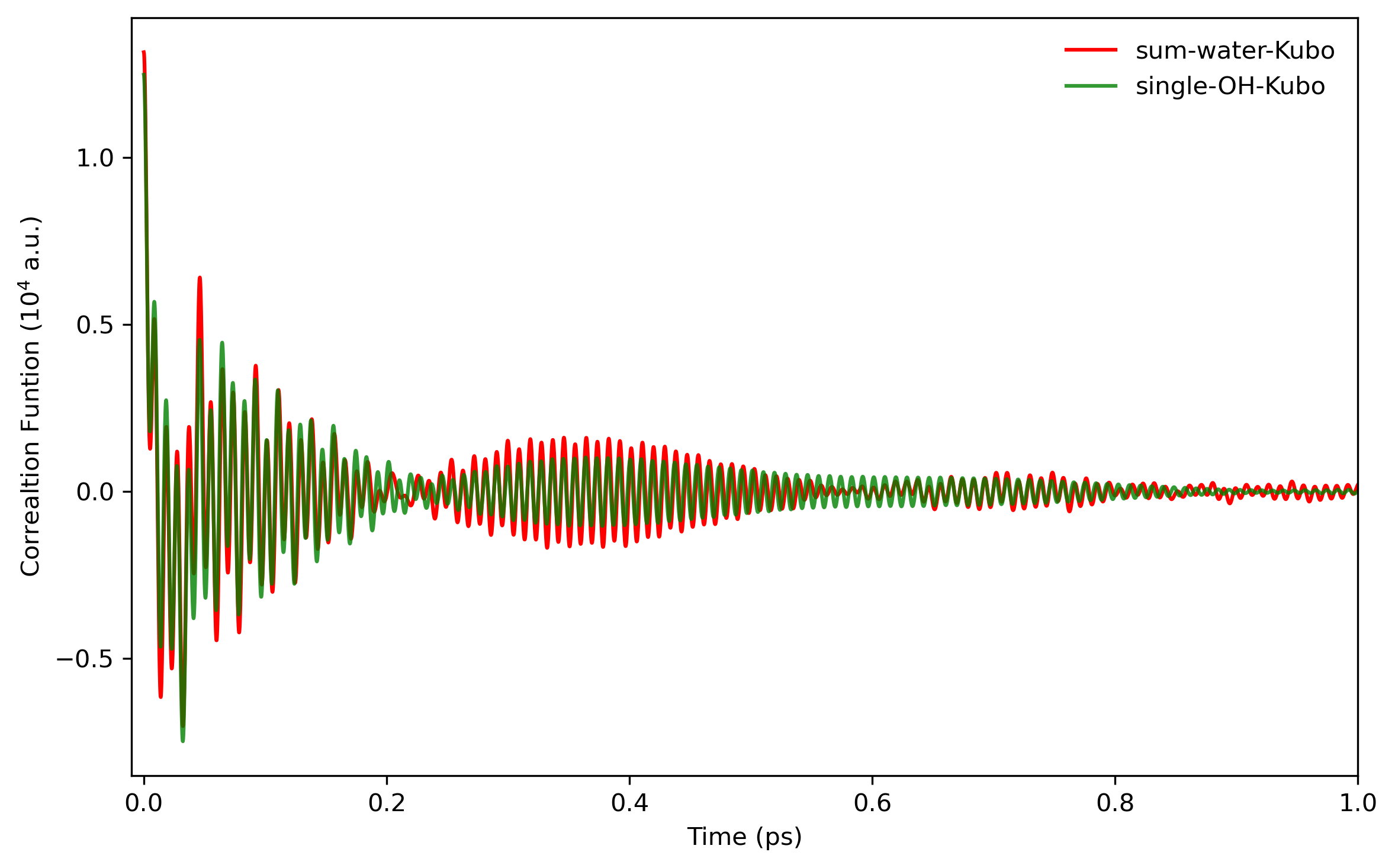
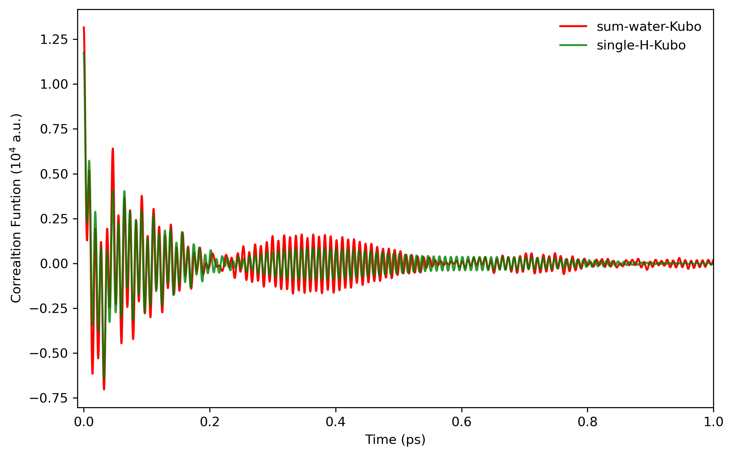
The self-diffusion constant of a single water molecule can be obtained from the center-of-mass momentum autocorrelation function:
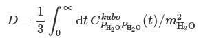
Here, center-of-mass momentum autocorrelation function corresponds to the sixth column of data in ‘LSC_cor-216-vv.dat’ file. The awk command can be used to get the 6th column from the data file:
$ awk 'NF>1{print $6}' LSC_cor-216-vv.dat > 6.datSince the oxygen atom is much heavier than the hydrogen atom, a reasonable way is to use the oxygen momentum autocorrelation function to calculate the diffusion constant. Here is a comparison of the two kinds of correlation functions (results with 8000 trajectories), see also Fig. 6. in Liu et al.

The integration of the correlation functions can be computed numerically. For example, the Trapezoidal rule can be used. The result value of diffusion constant will be around 0.50 if converged.
4.5.2 Infrared spectrum
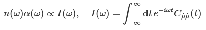
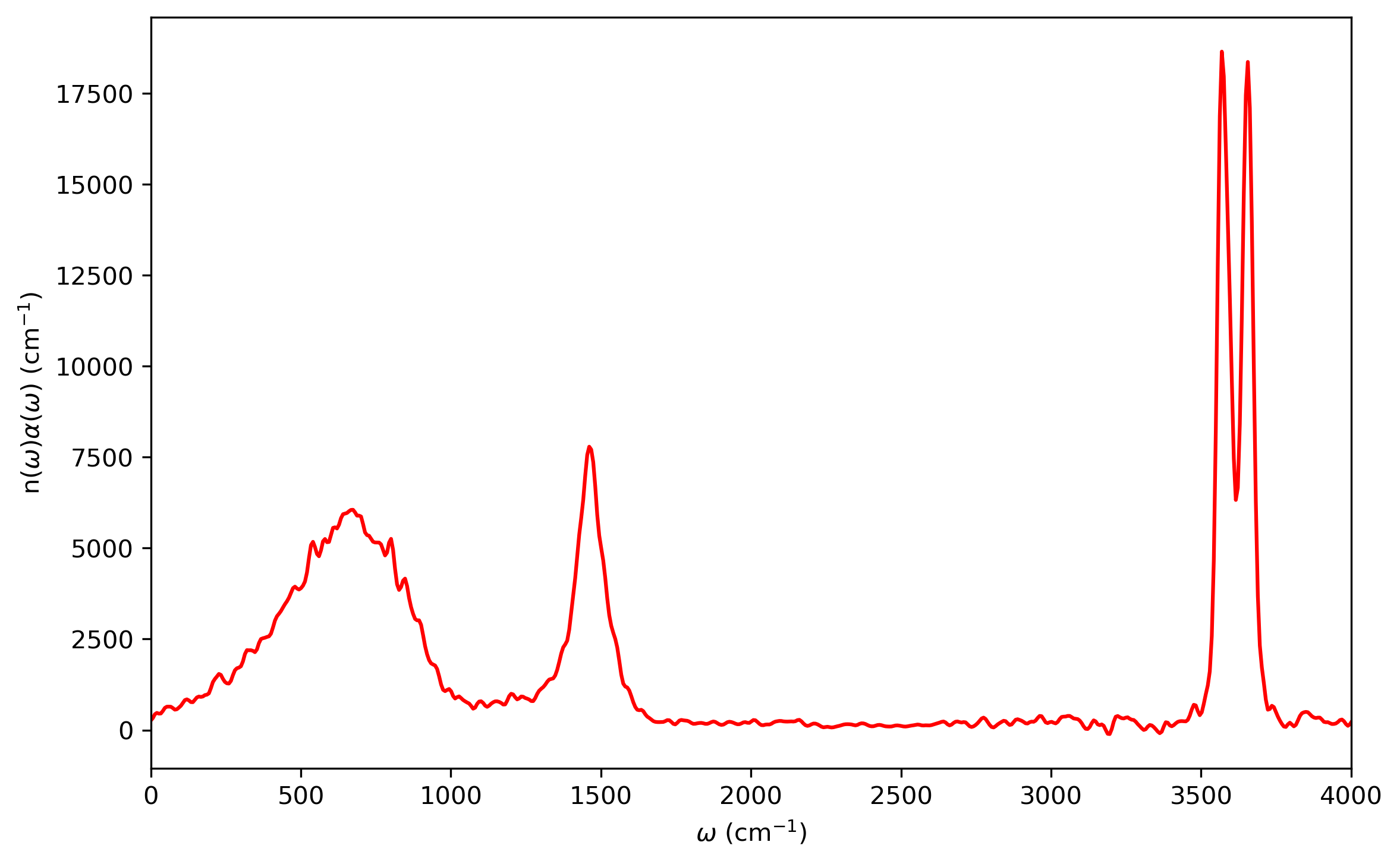
The experimental IR spectrum is given in terms of two frequency-dependent properties, the Beer-Lambert absorption constant α(ω) and the refractive index n(ω). These quantities are directly related to the dipole-derivative absorption line shape by
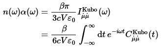
The infrared intensities along with the frequencies are obtained by Fourier transformation using the (dipole-derivative)-(dipole-derivative) Kubo-transformed correlation function, which is the fifth column of the ‘LSC_cor-216-vv.dat’ file. One can get the values from the data file by running the awk command in the terminal:
$ awk 'NF>1{print $5}' LSC_cor-216-vv.dat > 5.dat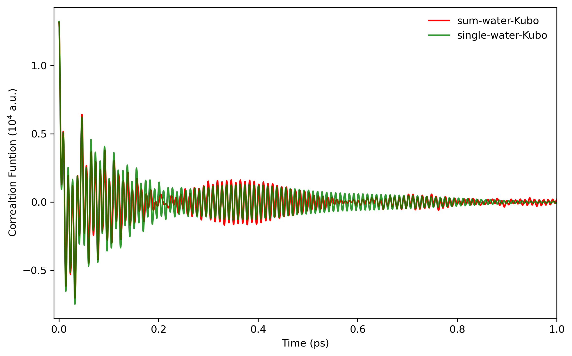
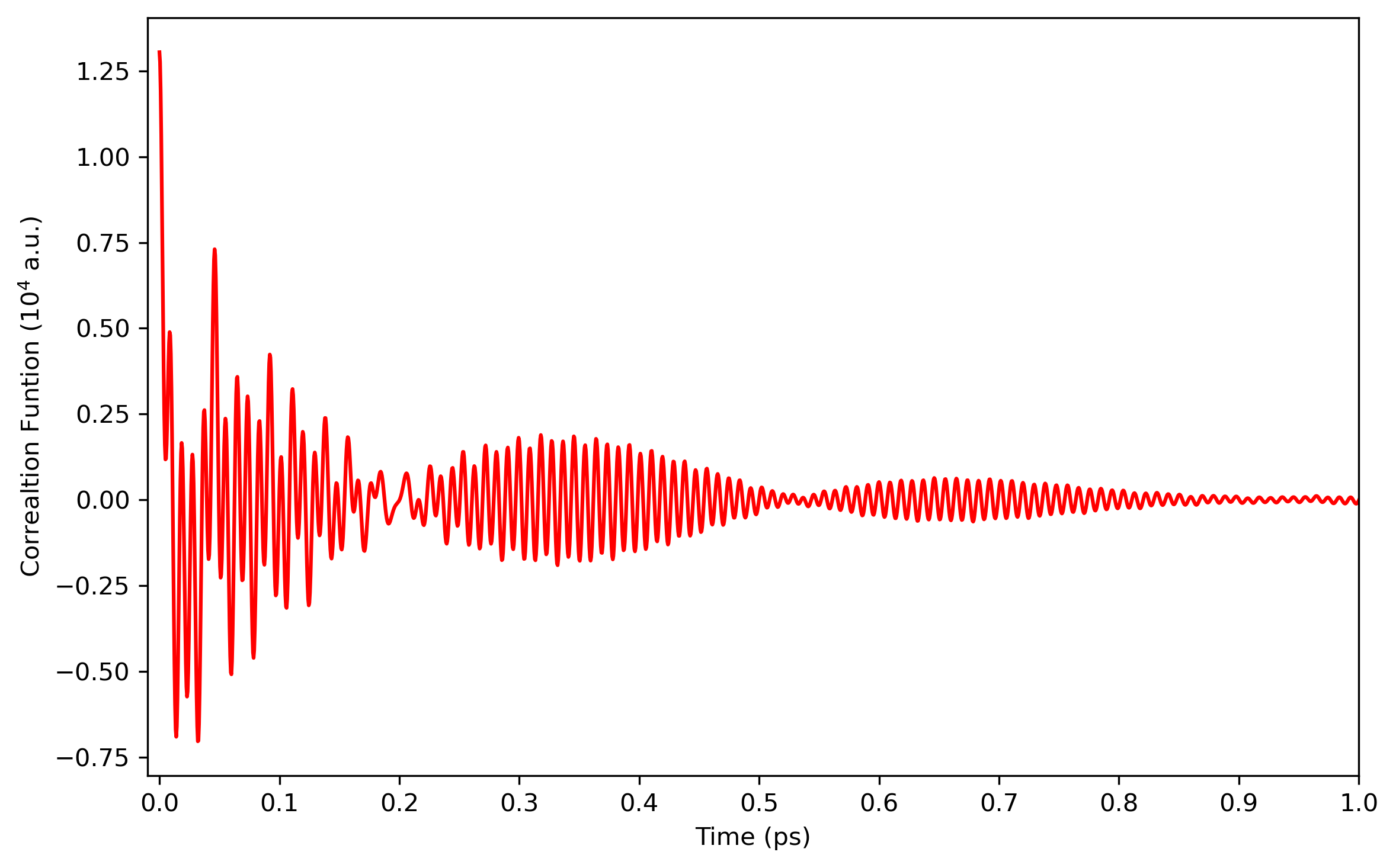
Fourier transformation is performed to obtain the infrared intensities. The infrared spectrum will be like
5. Results and Discussion
5.1 Velocity and bond length distributions

We first consider the configuration distribution (e.g. O-H bond length distribution) and velocity distribution (e.g. hydrogen atom velocity distribution) of MD and PIMD before sampling. We can see from Fig. 5.1 and Fig. 5.2 that PIMD results have broader distribution than those of MD, since the density distribution in Wigner phase space is given by:
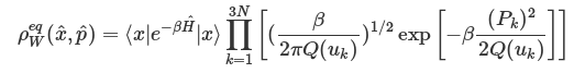
where uk = βℏωk,Pk is the k-th component of the mass-weighted normal mode momentum P and the quantum correction factor with the LGA ansatz proposed by Liu and Miller for both real and imaginary frequencies is given by:
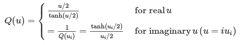
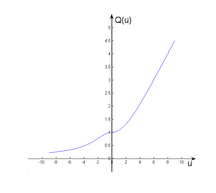
When u > 0, Q(u) > 1 (see Fig. 5.3), so the width of distribution will become broader.
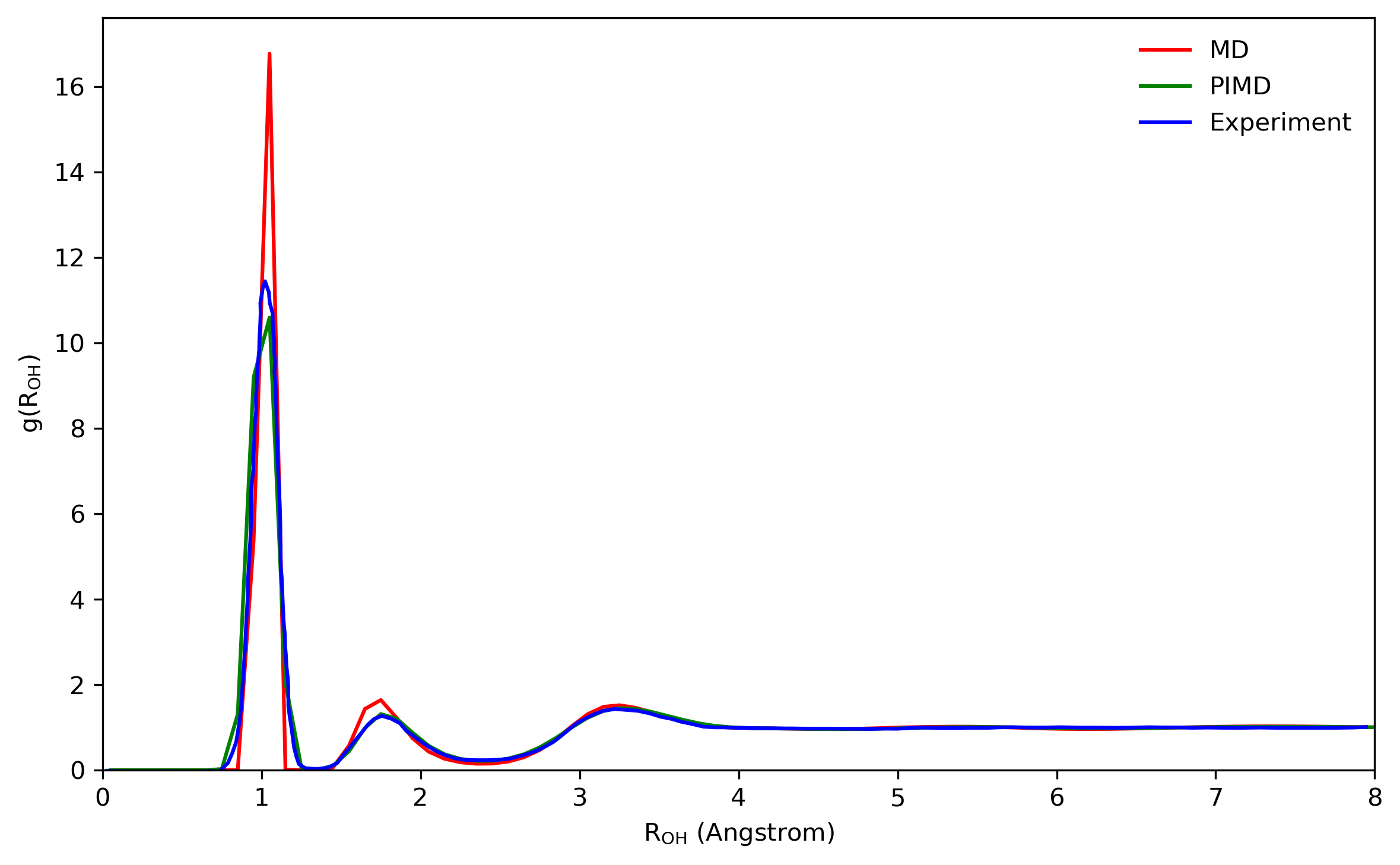
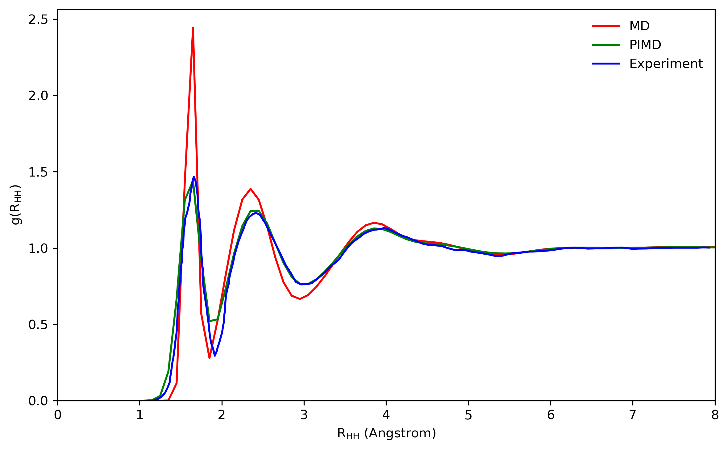
5.2 Radial distribution functions
The radial distribution functions (RDFs) computed with the q-SPC/fw model using the PIMD method are compared with the corresponding classical and experimental results as shown in Fig. 5.4. By comparing both the height and the position of peaks, it is shown that quantum RDFs agree better with the experimental results than classical results. The results computed here are also compared with reference values

5.3 About correlation functions
The LSC-IVR formulation of the quantum correlation function is
\[ C_{AB}(t) = \int \frac{1}{Z} \left<\mathbf{x}_0\right|e^{-\beta\hat{H}}\left|\mathbf{x}_0\right> \left|\frac{2\pi}{\beta}\mathbf{M}_\text{therm}(\mathbf{x}_0)\right|^{-1/2} \exp \left[-\frac{\beta}{2} \mathbf{p}_0^T \mathbf{M}_\text{therm}^{-1}(\mathbf{x}_0) \mathbf{p}_0 \right] \ f_{A^\beta}^W (\mathbf{x}_0,\mathbf{p}_0) B_W (\mathbf{x}_t,\mathbf{p}_t) d\mathbf{x}_0 d\mathbf{p}_0 \]
Here, the thermal mass matrix is given by \(\mathbf{M}_\text{therm}=\mathbf{M}^{1/2} \mathbf{T} \mathbf{Q} \mathbf{T}^T \mathbf{M}^{1/2}\) in the LGA ansatz, where \(\mathbf{M}\) is the diagonal mass matrix, \(\mathbf{T}\) is the orthogonal matrix that diagonalized the mass-weighted Hessian matrix of the PES
\[ \mathbf{T}^T \mathbf{M}^{-1/2} \frac{\partial^2 V }{ \partial \mathbf{x}^2} \mathbf{M}^{-1/2} \mathbf{T} = \text{diag}\left\{\omega_1^2,\cdots,\omega_{3N}^2\right\} \]
And \(\mathbf{Q}\) is a diagonal matrix whose elements are quantum correction factors discussed above \(\mathbf{Q} = \text{diag}\left\{ Q(\beta\hbar\omega_1),\cdots,Q(\beta\hbar\omega_{3N})\right\}\). \(f_{A^\beta}^W\) and \(B_W\) are functions depend on operators \(\hat{A}\) and \(\hat{B}\).
For the center-of-mass momentum correlation function, the center-of-mass momentum is a linear function of momentum. So does the dipole-derivative in the point charge model. In these cases, the LSC-IVR formulation of the Kubo-transformed correlation function is
\[ C_{\dot{A}\dot{A}}^\text{Kubo}(t) = \int \frac{1}{Z} \left<\mathbf{x}_0\right|e^{-\beta\hat{H}}\left|\mathbf{x}_0\right> \left|\frac{2\pi}{\beta}\mathbf{M}_\text{therm}(\mathbf{x}_0)\right|^{-1/2} \exp \left[-\frac{\beta}{2} \mathbf{p}_0^T \mathbf{M}_\text{therm}^{-1}(\mathbf{x}_0) \mathbf{p}_0 \right] \ \left(\frac{\partial A}{\partial \mathbf{x}}\right)^T \mathbf{M}_\text{therm}^{-1}(\mathbf{x}_0) \mathbf{p}_0 \ \left(\frac{\partial A}{\partial \mathbf{x}}\right)^T \mathbf{M}^{-1} \mathbf{p}_t \ d\mathbf{x}_0 d\mathbf{p}_0 \]
where \(A\) can be the components of center-of-mass coordinate or dipole moment, and \(\partial A/\partial \mathbf{x}\) is constant. Therefore, we only need to save the initial thermal velocity \(\mathbf{v}_\text{therm} \equiv \mathbf{M}_\text{therm}^{-1}(\mathbf{x}) \mathbf{p}\) for each LSC-IVR trajectory and velocity \(\mathbf{v} = \mathbf{M}^{-1}\mathbf{p}\) at each step of each LSC-IVR trajectory for calculating these correlation functions.
However, for general dipole moment surfaces, the dipole moment may be a nonlinear function of coordinate. In this case, the LSC-IVR formulation of the dipole-derivative correlation function can be expressed as
\[ C_{\dot{A}\dot{A}}^\text{Kubo}(t) \approx \int \frac{1}{Z} \left<\mathbf{x}_0\right|e^{-\beta\hat{H}}\left|\mathbf{x}_0\right> \left|\frac{2\pi}{\beta}\mathbf{M}_\text{therm}(\mathbf{x}_0)\right|^{-1/2} \exp \left[-\frac{\beta}{2} \mathbf{p}_0^T \mathbf{M}_\text{therm}^{-1}(\mathbf{x}_0) \mathbf{p}_0 \right] \ \left(\frac{\partial A}{\partial \mathbf{x}_0}\right)^T \mathbf{M}_\text{therm}^{-1}(\mathbf{x}_0) \mathbf{p}_0 \ \left(\frac{\partial A}{\partial \mathbf{x}_t}\right)^T \mathbf{M}^{-1} \mathbf{p}_t \ d\mathbf{x}_0 d\mathbf{p}_0 \]
where \(A\) can be the components of dipole moment whose analytical derivative may be complicated to obtain. It is more efficient to estimate the term \(\left(\partial A/\partial \mathbf{x}\right)^T \mathbf{M}_\text{therm}^{-1}(\mathbf{x}) \mathbf{p}\) by using the finite difference scheme
\[ \left(\frac{\partial A}{\partial \mathbf{x}}\right)^T \mathbf{M}_\text{therm}^{-1}(\mathbf{x}) \mathbf{p} \approx \frac{A\left(\mathbf{x} + \varepsilon \mathbf{M}_\text{therm}^{-1}(\mathbf{x}) \mathbf{p}\right) - A\left(\mathbf{x} - \varepsilon \mathbf{M}_\text{therm}^{-1}(\mathbf{x}) \mathbf{p}\right) }{2\varepsilon} \]
where \(\varepsilon\) is a small quantity to guarantee the convergence. \(\varepsilon\) should be adjusted as the vector \(\mathbf{M}_\text{therm}^{-1}(\mathbf{x}) \mathbf{p}\) varies. A reasonable choice could be
\[ \varepsilon = \frac{\delta x}{\left\|\mathbf{M}_\text{therm}^{-1}(\mathbf{x}) \mathbf{p}\right\|} \]
where \(\delta x\) is a small constant parameter depend on the system and \(\left\|\mathbf{M}_\text{therm}^{-1}(\mathbf{x}) \mathbf{p}\right\|\) represents the length of the vector \(\mathbf{M}_\text{therm}^{-1}(\mathbf{x}) \mathbf{p}\). Note that such finite difference only need to be computed for the initial condition of each LSC-IVR trajectory. For the dipole-derivative at time \(t\), \(\left(\partial A / \partial \mathbf{x}_t\right)^T \mathbf{M}^{-1} \mathbf{p}_t = \dot{A} \left(\mathbf{x}_t,\mathbf{p}_t\right)\), the finite difference \([A(t+\Delta t)-A(t-\Delta t)]/2\Delta t\) along the real-time trajectory can be used if the real-time stepsize is relatively small.
5.4 Diffusion constant
As shown in Table 5.1, the diffusion constant computed with classical dynamics is 0.18, while the diffusion constant given by LSC-IVR with PIMD sampling is 0.50. Both of these two results are consistent with those from the reference we cited, respectively. However, one should note that direct comparison between the result of LSC-IVR and that of experiment makes no sense, since the diffusion constant, as one of the dynamic properties, was selected to optimize the parameters of the q-SPC/fw model, which was originally used in CMD calculation to reproduce the experimental value.
Note: the results listed in the table below are calculated from 8000 trajectories in a single simulation, which is insufficient to get an error bar.
| Method | Calc. | Ref. |
|---|---|---|
| Classical | 0.18 | 0.18±0.01 |
| Quantum | 0.50 | 0.50±0.01 |
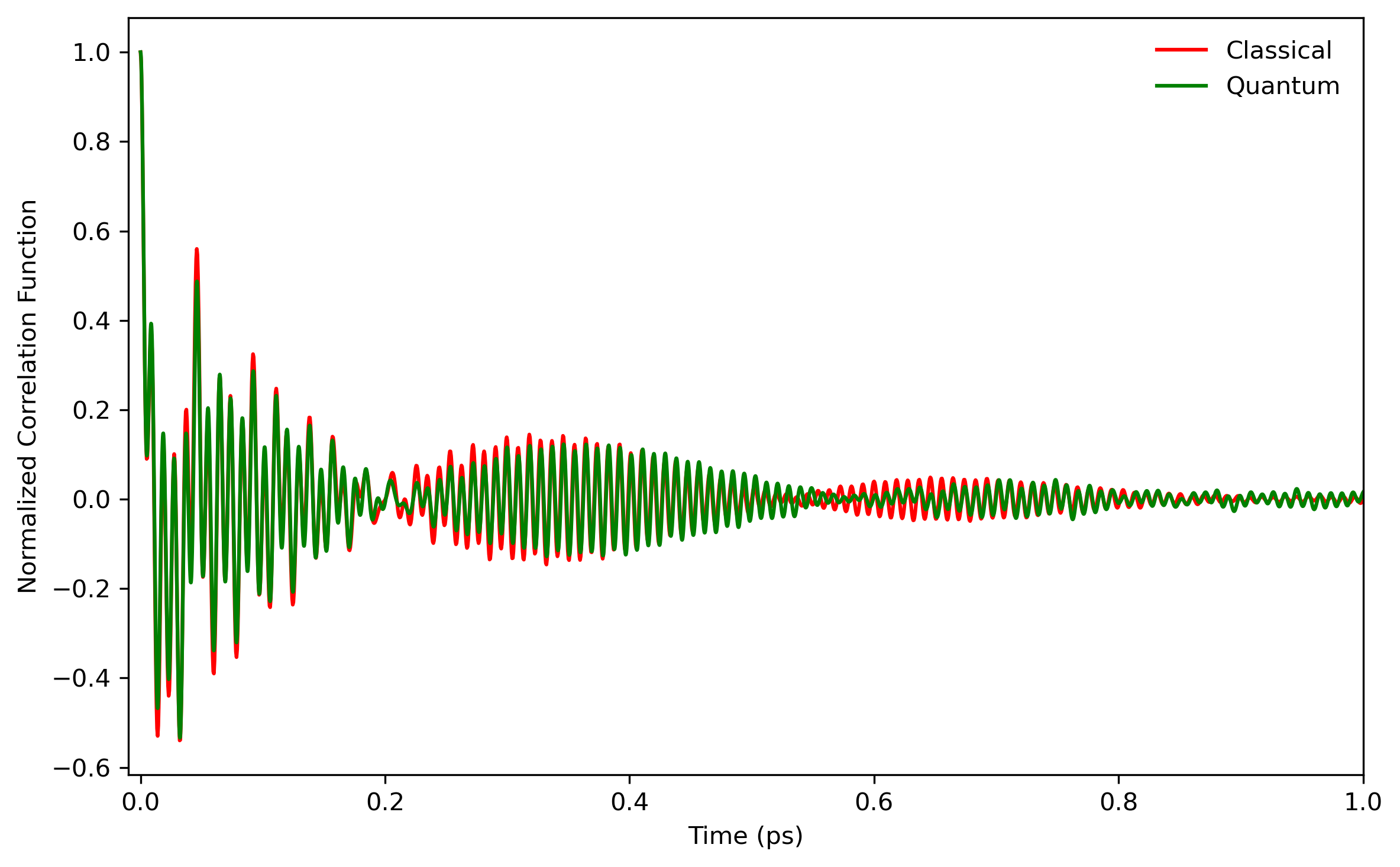
The comparison of the (normalized) velocity autocorrelation functions obtained from classical and quantum dynamics can also been seen in Fig. 5.5.

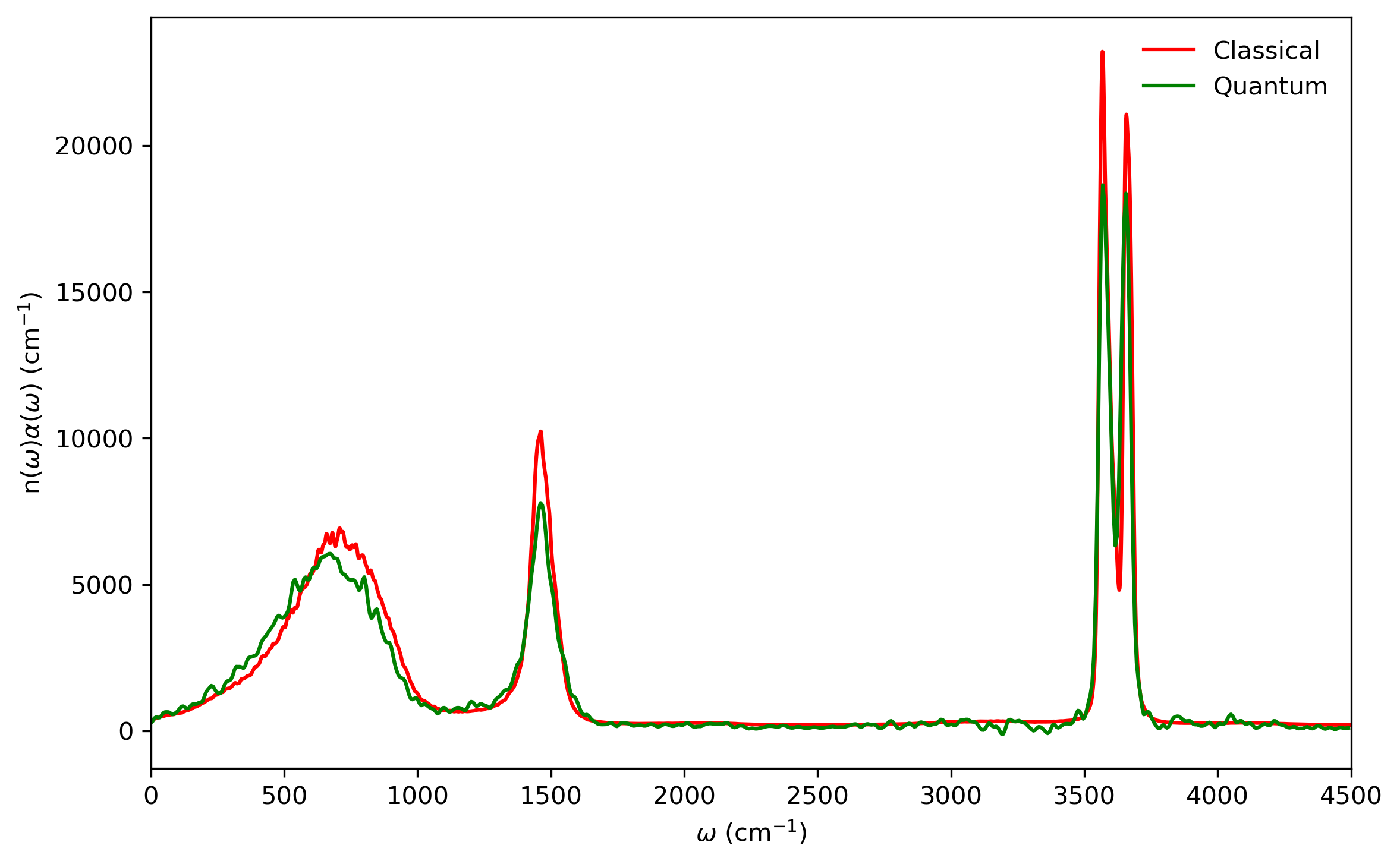
5.5 Infrared spectrum
Fig. 5.6 shows the comparison of LSC-IVR dipole-derivative correlation functions with those of classical MD method. These two results are rather similar, except that the LSC-IVR result predicts a more rapid decay of the amplitude and longer oscillation periods of the correlation function than that is seen in classical MD simulation.
6. Appendix
6.1 Test of parameters in the NPT ensemble for classical dynamics
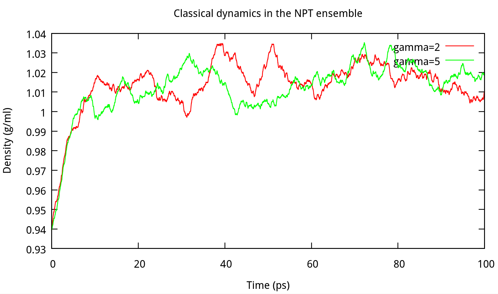
6.1.1 gamma_ln for Langevin dynamics
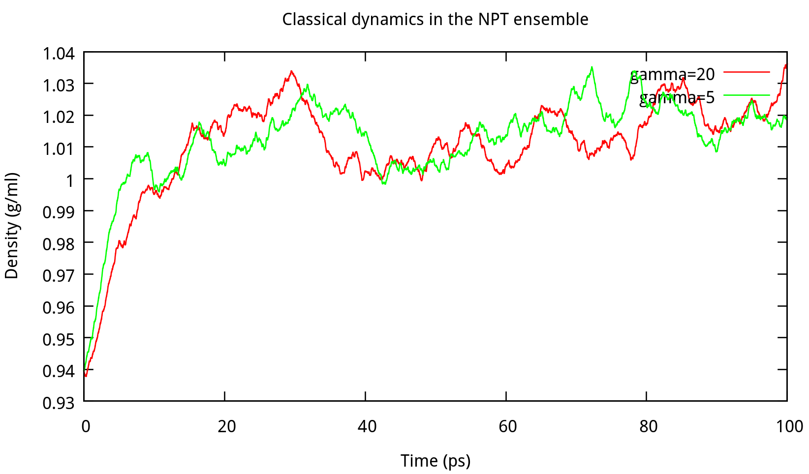
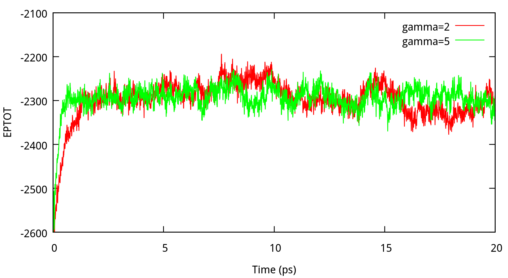
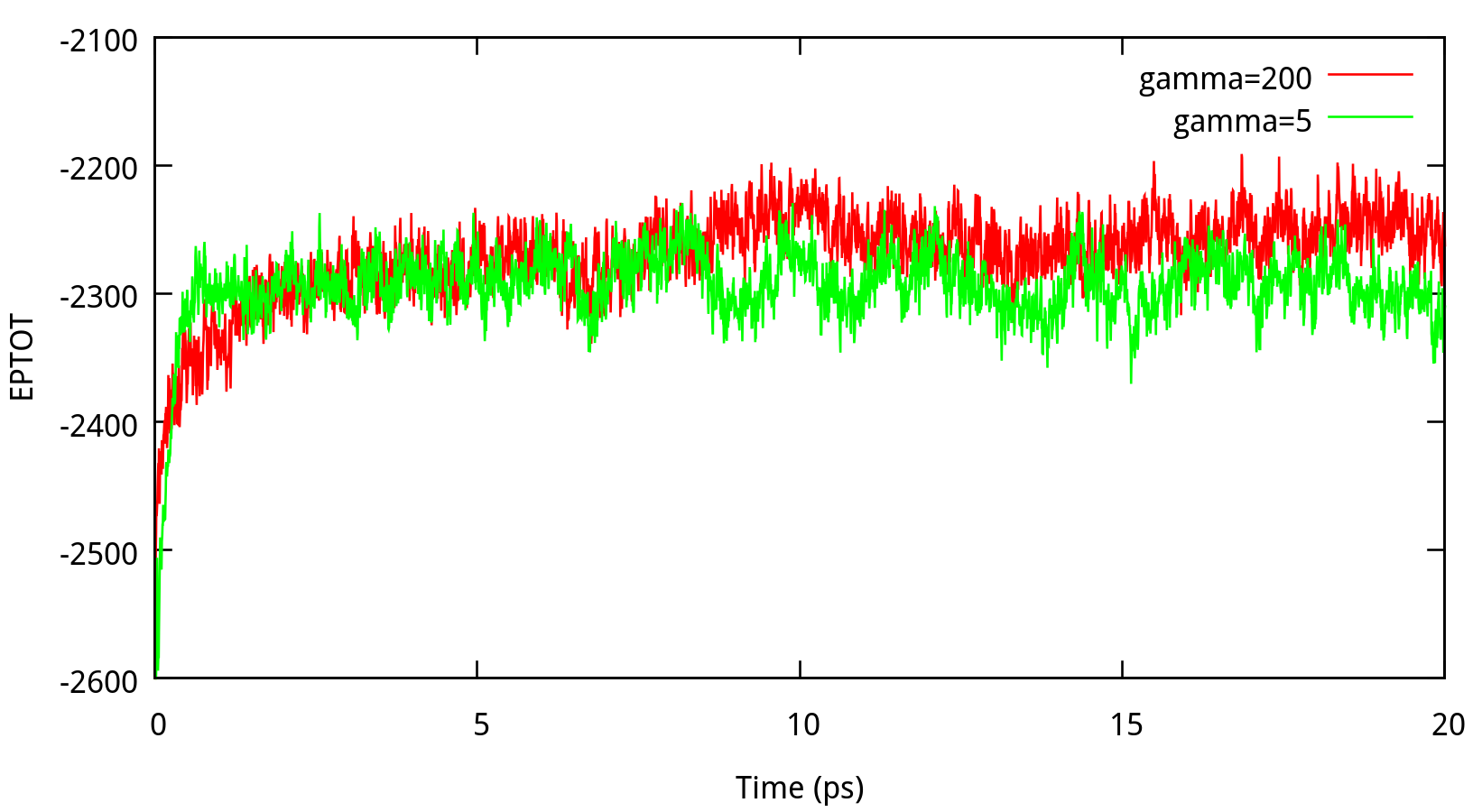
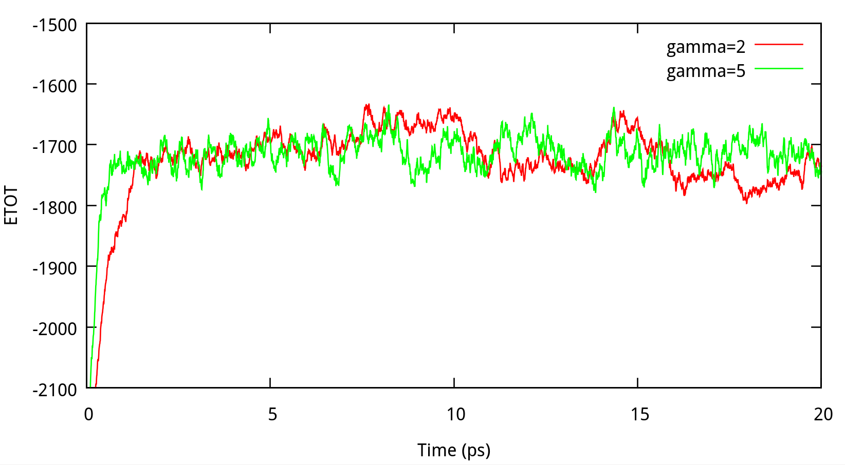
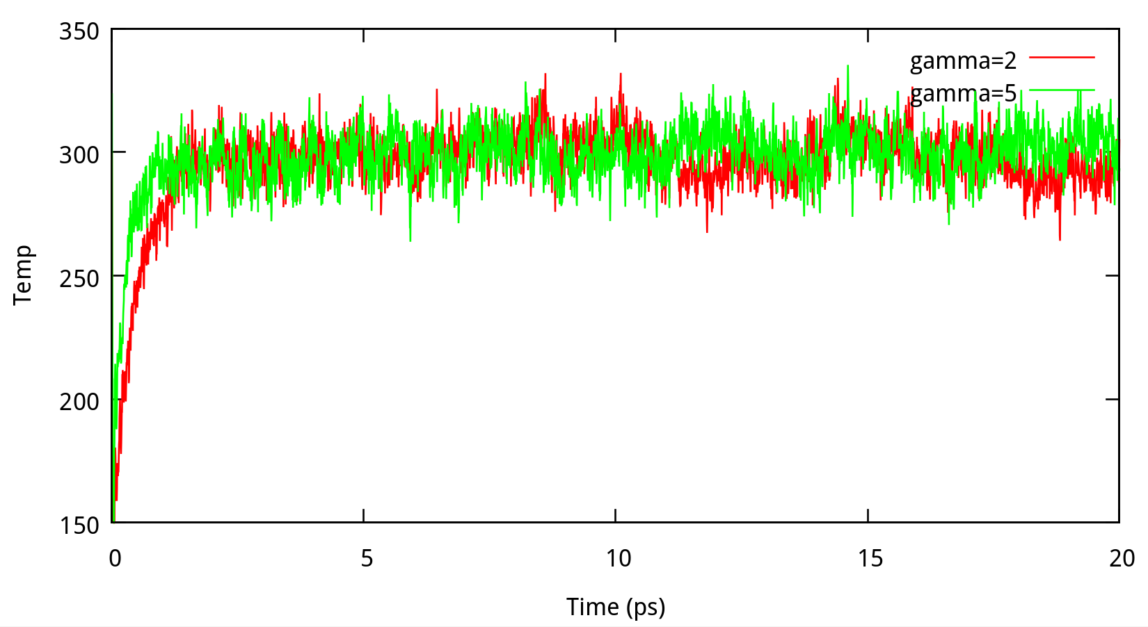
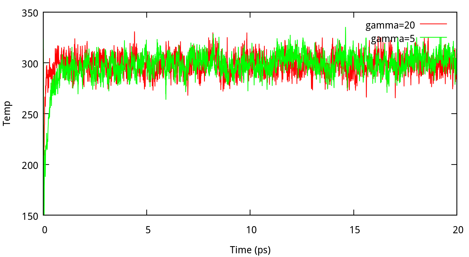
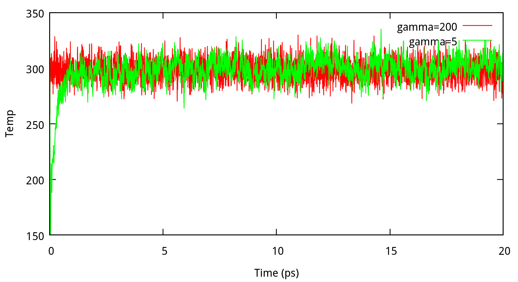
In classical dynamics, Langevien thermostat (ntt=3) is used to maintain the temperature of the liquid system at 298.15K. This temperature control method uses Langevin dynamics with a collision frequency given by gamma_ln (in ps-1). As Amber Reference Manual says, it is not necessary that gamma approximates the physical collision frequency, which is about 50 ps-1 for liquid water. Here we give the results about tests of gamma in the NPT ensemble in Figure 6.1. Clearly, we can see that too small and too large values of gamma_ln will lead to a big fluctuation of temperatures and energies, and the value of gamma_ln around 5 – 20 ps-1 is suitable for the system here.


6.1.2 taup for NPT simulation
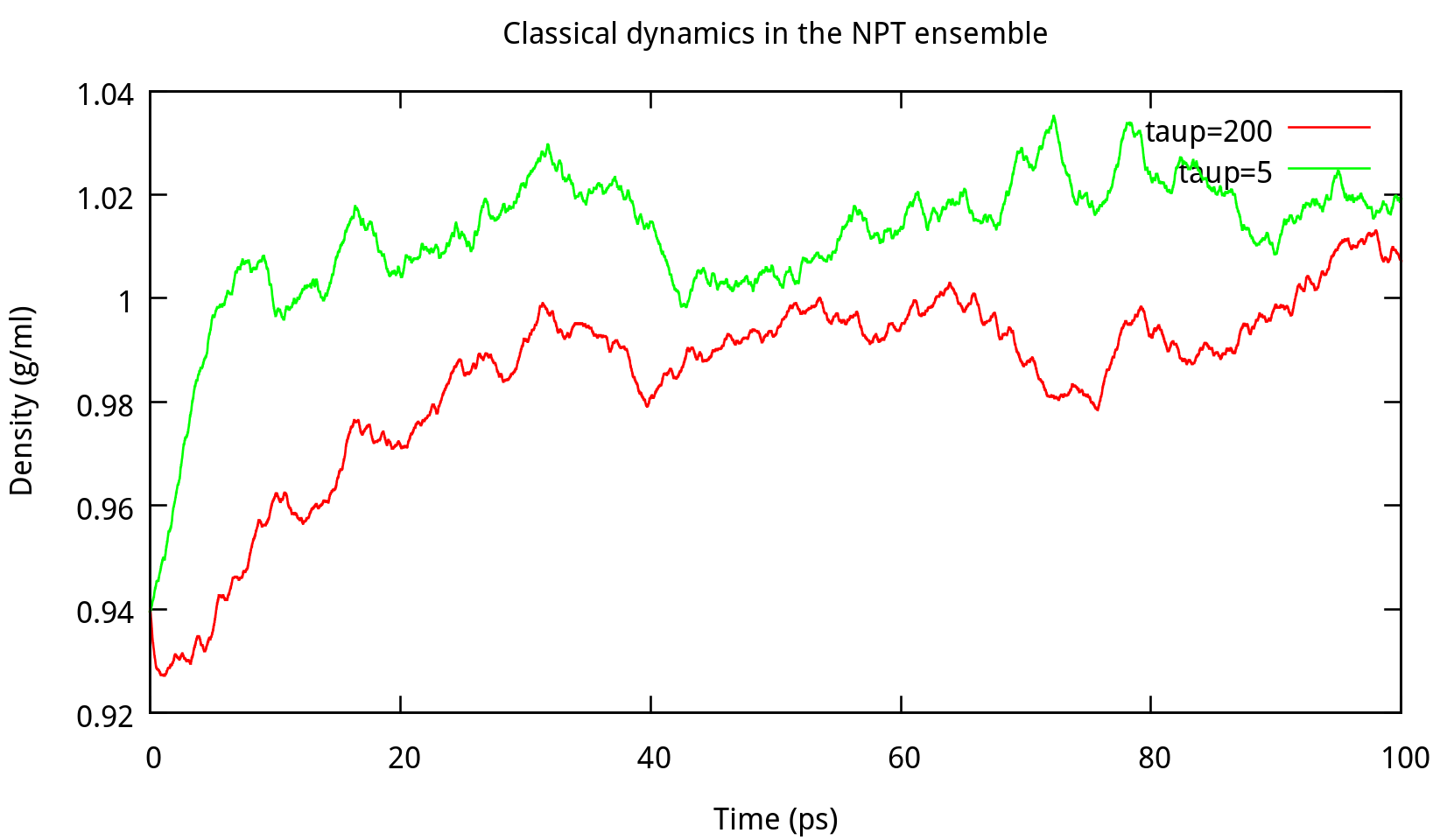
In ‘constant pressure’ dynamics, taup is used to define the pressure relaxation time (in ps). The recommended value is between 1.0 and 5.0 ps as Amber Reference Manual says. Here are some testing results:
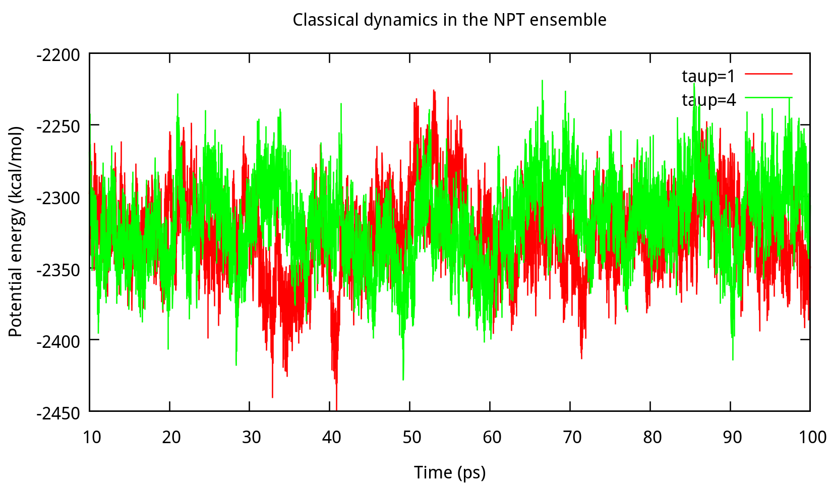
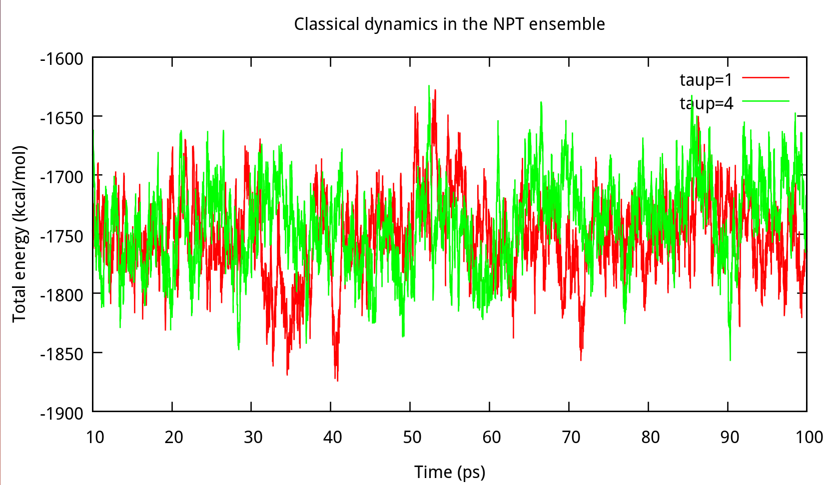
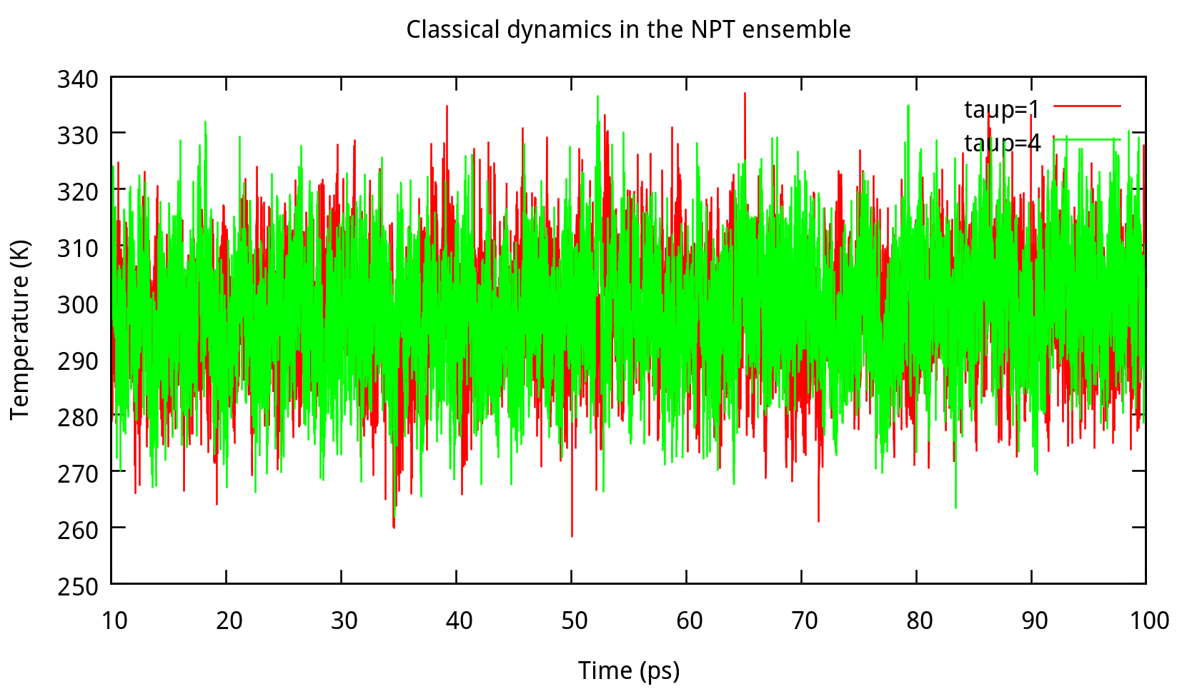
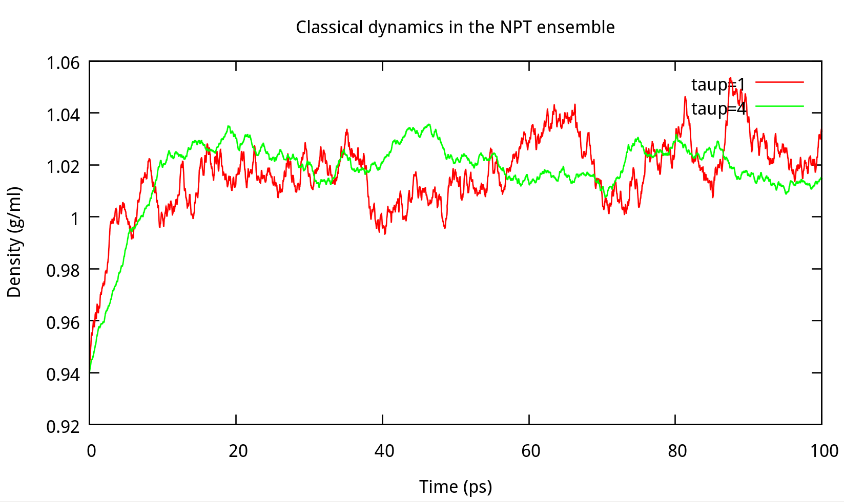
taup in the NPT ensemble. The results of potential energy, total energy, temperature, and density.Our results gives the comparison of the density, temperature and energy information at
taup=1 and taup=4 for the liquid water system in Figure 6.2. In this work, taup=1 and taup=4 simulation give almost the same fluctuation around a constant mean value for temperature, potential energy and total energy, however, the latter one seems to be more stable in density. Thus, taup=4 is used for classical dynamics in the NPT ensemble.
6.2 Test of parameters for PIMD simulation
6.2.1 Number of beads and size of time step
One must be mentioned at the outset that no quantum dynamical properties can be generated using the techniques in normal classical MD methods. Fortunately, the formulation by Feynman of quantum statistical mechanics in terms of path integrals has provided us the ability to analyze the properties of quantum many-body systems at finite temperature. The continuous functional representation of the path integral is mathematically elegant, however, it is not suitable for direct numerical evaluation. The classical isomorphism known as the connection between quantum system and the P-particle fictitious classical system (Fig. 6.3) can evaluate the numerical evaluation by applying the equations of motion derived from fictitious Hamiltonian to classical MD methods.
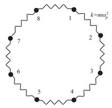
Generally speaking, the more the number of beads in fictitious classical system is, the better will fictitious classical system describe quantum system. In practice this is not possible. A suitable size of P (the number of beads) combined computational efficiency and accuracy is important. Energies are computed in PIMD simulation with various P and time steps, to obtain an optimal P and a suitable time step (dt).
| P | dt | V | ρ |
|---|---|---|---|
| 1 | 0.5 | -2326.50 ± 5.65 | 1.0177 ± 0.0011 |
| 12 | 0.125 | -1204.74 ± 3.68 | 0.9999 ± 0.0021 |
| 24 | 0.1 | -1050.15 ± 4.05 | 0.9996 ± 0.0016 |
| 36 | 0.05 | -1011.45 ± 5.18 | 0.9987 ± 0.0016 |
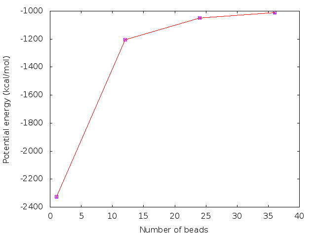

From the above tables and figures, it is clear that 24 beads with the choice of time step of 0.1 fs is sufficient for convergence of potential energies and densities obtained from the PIMD simulation.
6.2.2 Number of Nosé-Hoover chains of thermostats
The averages obtained in a conventional MD simulation are equivalent to ensemble averages in the microcanonical (constant-NVE) ensemble instead of canonical ensemble. Several technologies implemented to perform MD simulation at constant temperature could generate a canonical distribution. As recommended in Amber 12 Reference Manual, Nosé-Hoover chains of thermostats is implemented for NMPIMD (ipimd=2) in this tutorial. More Nosé-hoover chains of thermostats leads to more stable temperature, but also more computation burden. Therefore, the determination of chain’s number also need to be careful. The choice of an appropriate number of chains depends on the system. Typically, 4 chains of thermostats (nchain=4) are sufficient to guarantee an efficient sampling of the phase space. Here are some testing results:
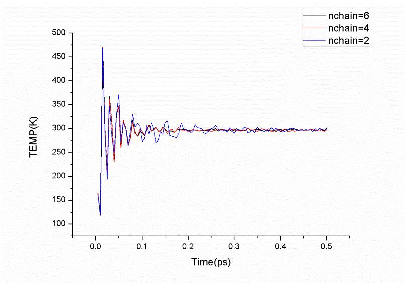
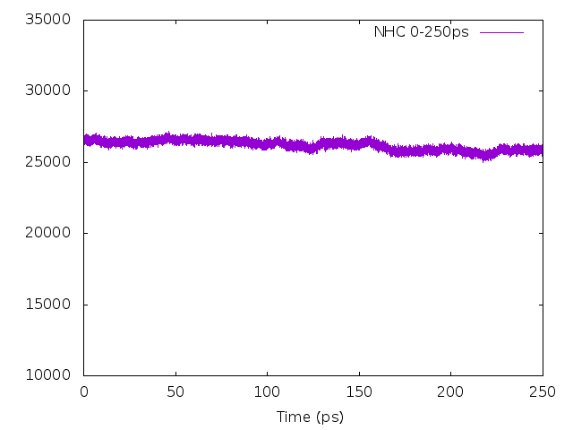
As shown in Figure 6.5, the fluctuation of the temperature for the system with 2 chains of thermostats is larger than that of 4 chains and 6 chains before equilibrium, while systems with 4 chains and 6 chains give almost the same fluctuation in temperature before equilibrium and the same density distribution in 200 ps after equilibrium. Based on these, 4 chains of thermostats would be an optimal choice for an efficient sampling of the phase space. Moreover, note that you must carefully check the timestep used in the simulation, which should be small enough to guarantee conservation of the energy of the extended system of the Nosé-Hoover chains of thermostats. From Figure 6.6, we can see that
dt=0.0001 (ps) is a suitable choice.
6.3 Using gnuplot in analysis
gnuplot is a free, command-driven, interactive, function and data plotting program. It is used to plot most figures in this tutorial. In this section, we introduce two examples of gnuplot usage, one plots the figure with two columns of data as x and y respectively, the other plots the distribution of the second column of data. For more details, please refer to the help files of gnuplot and search engine.
6.3.1 Plotting a figure with data file
gnuplot can be used interactively by type gnuplot in terminal:
$ gnuplotthen type the following commands in the gnuplot interface:
gnuplot> set term png enhanced
gnuplot> set output 'HH-distance.png'
gnuplot> set xlabel 'nstep'
gnuplot> set ylabel 'H-H (Angstrom)'
gnuplot> plot 'HH-distance.dat' using 1:2 with points title 'HH-distance'
Note: type the stuff after ‘gnuplot>’ then hit ‘Enter’.
A figure will be created as below:
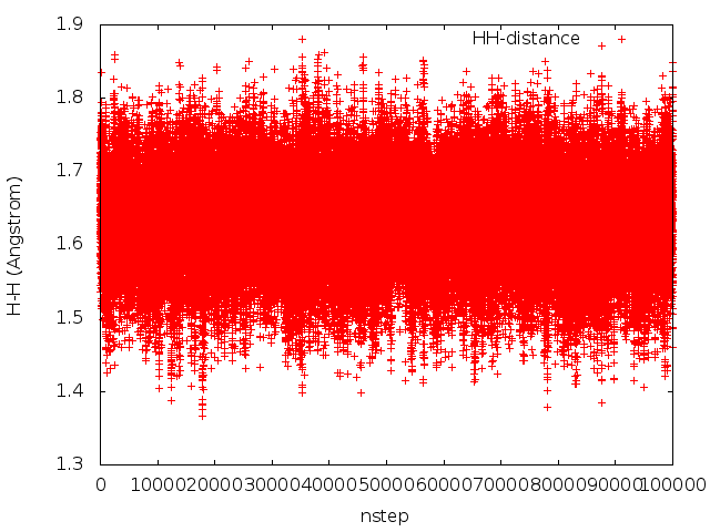
Here is the example input data file HH-distance.dat.
One can also plot the figure without entering the gnuplot interface. First write the gnuplot commands in a text file, say, plot.gnu, then run the command in terminal:
$ gnuplot plot.gnuThe same figure will be obtained as above.
6.3.2 Plotting distribution of data
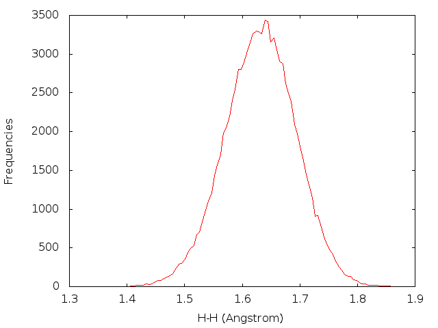
We do almost the same thing as gnuplot Frequency Plot except the setting of ‘bin_width’. A shell script is used to get the minimum and maximum value of data, then ‘bin_width’ is computed as separating the values into 100 intervals.
#!/bin/bash

f="HH-distance.dat"
v="H-H"
list=(`awk '{print $2}' $f | sort -n`)
min=${list[0]}
max=${list[${#list[@]}-1]}

# write the file for gnuplot
echo "set term png enhanced

set output 'dist_${v}.png'
set xlabel '${v} (Angstrom)'
set ylabel 'Frequencies'
min=$min
max=$max
bin_width=(max-min)/100.;     # set bin width
bin_num(x)=floor(x/bin_width)
rounded(x)=bin_width*(bin_num(x) + 0.5)
plot '${f}' u (rounded(\$2)):(1) t '' smooth frequency with lines
" |  gnuplot
Then a figure named ‘dist_H-H.png’ will be plotted.
6.4 Using ptraj in analysis
As one of the main analysis code for Amber, ptraj is a program to process and analyze a series of 3-D atomic coordinates (one molecular configuration or frame at a time). In this tutorial, it is used to calculate radial distribution functions (RDFs), bond-lengths and bond-angles from the trajectory file.
6.4.1 Calculating radial distribution function
In order to calculate the radial distribution funtions (RDFs), ptraj is used to analyze sets of 3-D coordinates from trajectory file ‘mdcrd’. In the liquid water, we will calculate the RDFs of the H and O atoms.
First, we create an input file ptraj_rdf.in
trajin mdcrd
radial O-H 0.05 9.0 :WAT@O :WAT@H1,H2
radial H-H 0.05 9.0 :WAT@H1 :WAT@H1,H2
radial O-O 0.05 9.0 :WAT@O :WAT@O
Here, ‘O-H’, ‘H-H’ and ‘O-O’ are the headers for output file names, respectively; 0.05 is the bin size, 9.0 is the maximum for the histogram, and :WAT@O is the mask for selecting atoms we want to use for our analysis. Then, run this command in terminal:
$ ptraj wat216.prmtop ptraj_rdf.inThe output file after running the ptraj_rdf.in file will be:
O-H_standard.xmgr, O-H_volume.xmgr, O-H_carnal.xmgr,
H-H_standard.xmgr, H-H_volume.xmgr, H-H_carnal.xmgr,
O-O_standard.xmgr, O-O_volume.xmgr, O-O_carnal.xmgr.
Use gnuplot to plot the resulting graph of the RDFs, then we have the figures in Fig. 5.4.
6.4.2 Calculating bond and angle distribution
In the MD and PIMD NVT stages, it is recommended that the bond and angle distribution of the trajectory should be checked. Here, we can still use ptraj script to collect the bond length and angles along the trajectory.
Here is an example of input file ptraj_dist.in:
trajin mdcrd
distance H2-H1 @3 @2 out HH-distance.dat
angle H1-O-H2  @2 @1 @3 out HOH-angle.dat
Note: the residue
:WATcannot be included in the mask for selecting atoms
Then, run this command in terminal:
$ ptraj wat216.prmtop ptraj_dist.inThe output file after running the ptraj_dist.in file will be: ‘HH-distance.dat’, and ‘HOH-angle.dat’.
Then gnuplot is used to plot the distribution of data in these files, just like what’s done in the 6.3.2 section.
Note:
Do the following to obtain all necessary files for the tutorial.$ git clone https://github.com/jianliugroup/LSC-IVR-Amber.gitReferences
In addition to the paper,
Jian Liu, William H. Miller, Francesco Paesani, Wei Zhang, and David Case, “Quantum dynamical effects in liquid water: A semiclassical study on the diffusion and the infrared absorption spectrum” Journal of Chemical Physics, 131, 164509 (2009) [pdf version]please refer to the following references for more detail about the LGA/LSC-IVR and its recent progress
Jian Liu, William H. Miller, “A simple model for the treatment of imaginary frequencies in chemical reaction rates and molecular liquids”, Journal of Chemical Physics, 131, 074113 (2009) [pdf version]
Jian Liu, William H. Miller, Georgios S. Fanourgakis, Sotiris S. Xantheas, Imoto Sho, and Shinji Saito “Insights in quantum dynamical effects in the Infrared spectroscopy of liquid water from a semiclassical study with an ab initio-based flexible and polarizable force field”, Journal of Chemical Physics, 135, 244503 (2011) [pdf version]
Jian Liu, "Recent advances in the linearized semiclassical initial value representation/classical Wigner model for the thermal correlation function", International Journal of Quantum Chemistry, 115(11), 657-670 (2015) [Cover of this issue. Invited contribution.] [pdf version]
Xinzijian Liu, Jian Liu, "Critical role of quantum dynamical effects in the Raman spectroscopy of liquid water", Molecular Physics, 116(7-8), 755-779 (2018) [Cover of this issue. Invited contribution.] Free eprints [arXiv preprint] [pdf version]