Tutorial for CPU & GPU - The unified “middle” thermostat and barostat scheme in AMBER for efficient configurational sampling
Introduction
The tutorial offers an introduction to the unified “middle” scheme of thermostatting and barostatting algorithms in AMBER.
The prerequisites are listed as below:
- AMBER software package (2025 or later version) -
sanderand its parallel version,sander.MPI,pmemdand its parallel or GPU version,pmemd.MPI,pmemd.cuda_SPFPandpmemd.cuda_DPFP, are used to run simulations. In addition,LEaP(tleap and its graphical user interface, xleap) is utilized to generate the topology file of the simulated system.
The “middle” scheme offers a unified framework to develop efficient thermostatting and barostatting algorithms for configurational sampling for the canonical (NVT) ensemble and isothermal-isobaric (NPT) ensemble, as described in Refs. [1–5] [12] . It can be implemented for performing molecular dynamics (MD) or path integral molecular dynamics (PIMD), either with or without holonomic constraints. The “middle” scheme allows the use of much larger time intervals (i.e., time stepsizes) \(\Delta t\) to maintain the same accuracy, which significantly improves the configurational sampling efficiency. That is, it is efficient for calculating structural properties and thermodynamic observables that depend on coordinate variables (and the volume variable for the isothermal-isobaric ensemble).
When thermostatting algorithms are developed, most thermostats control the temperature by updating momenta of the system. Some prevailing thermostats include stochastic ones (such as the Andersen thermostat and Langevin dynamics) and deterministic ones (such as the Nosé-Hoover thermostat and Nosé-Hoover chain). In the “middle” scheme, immediately after the coordinate-updating step for half a time interval, the thermostat process for a full time interval takes place, which then followed by the coordinate-updating step for another half time interval [1,5] .
Here we present a brief introduction to the “middle” scheme. For many thermostats, the integration in one time step \(\Delta t\) can be splitted into three parts, the steps for updating coordinates, momenta and thermostat, denoted as “x”, “p” and “T”, respectively. In this case the “equations of motion” may be expressed as
\[ \begin{bmatrix} \mathrm{d}\mathbf{x}_t\\ \mathrm{d}\mathbf{p}_t \end{bmatrix} = \underbrace{ \begin{bmatrix} \mathbf{M}^{-1}\mathbf{p}_t\\ 0 \end{bmatrix}\mathrm{d}t }_{\text{x}} + \underbrace{ \begin{bmatrix} 0 \\ -\nabla_{\mathbf{x}_t}U(\mathbf{x}_t) \end{bmatrix}\mathrm{d}t }_{\text{p}} + \underbrace{ \begin{bmatrix} \text{thermostat} \\ \end{bmatrix} }_{\text{T}} \] (1) Here, \(U\) is the potential energy, \(\mathbf{M}\) is the diagonal mass matrix, \(\mathbf{x}\) and \(\mathbf{p}\) are the vectors of coordinate and momentum, respectively. Equation (1) is, however, not convenient to do the analysis.
A more useful approach is to employ the forward Kolmogorov equation to express the evolution of the density distribution in the phase space \(\rho(\mathbf{x},\mathbf{p})\) . \[ \begin{aligned} \frac{\partial}{\partial t}\rho =& \mathcal{L}\rho\\ =& (\mathcal{L}_{\text{x}} + \mathcal{L}_{\text{p}} + \mathcal{L}_{\text{T}})\rho \end{aligned} \] (2) The relevant Kolmogorov operators for the 1st and 2nd terms of the right-hand side (RHS) are \[ \mathcal{L}_{\text{x}}\rho = -\mathbf{p}^T\mathbf{M}^{-1}\nabla_{\mathbf{x}}\rho \] (3) \[ \mathcal{L}_{\text{p}}\rho = \nabla{}_{\mathbf{x}}U(\mathbf{x})\cdot\nabla{}_\mathbf{p}\rho \] (4) respectively. The definition of \(\mathcal{L}_{\text{T}}\) depends on the specific thermostat. The phase space propagators for a time interval \(\Delta t\) for the three parts are \(e^{\mathcal{L}_{\text{x}}\Delta t}\) , \(e^{\mathcal{L}_{\text{p}}\Delta t}\) , and \(e^{\mathcal{L}_{\text{T}}\Delta t}\) , respectively.
The propagation in each time step with the velocity Verlet (VV) algorithm is performed as \[ e^{\mathcal{L}\Delta t} \approx e^{\mathcal{L}^{\text{VV}}_{\text{middle}}\Delta t} = e^{\mathcal{L}_{\text{p}}\Delta t/2} e^{\mathcal{L}_{\text{x}}\Delta t/2} e^{\mathcal{L}_{\text{T}}\Delta t} e^{\mathcal{L}_{\text{x}}\Delta t/2} e^{\mathcal{L}_{\text{p}}\Delta t/2} \] (5) The phase space propagator for the thermostat part \(e^{\mathcal{L}_{\text{T}}\Delta t}\) is designed in the middle. Equation (5) is denoted as “VVMiddle”. The numerical algorithm reads \[ \begin{aligned} \text{Update Momenta for half a step:} \quad &\mathbf{p} \leftarrow \mathbf{p} - \frac{\partial U}{\partial \mathbf{x}} \frac{\Delta t}{2}\\ \text{Update Coordinates for half a step:} \quad &\mathbf{x} \leftarrow \mathbf{x} + \mathbf{M}^{-1}\mathbf{p} \frac{\Delta t}{2}\\ \text{Thermostat for a full time step:} \quad &\textit{thermostat_step} \\ \text{Update Coordinates for another half step:} \quad &\mathbf{x} \leftarrow \mathbf{x} + \mathbf{M}^{-1}\mathbf{p} \frac{\Delta t}{2}\\ \text{Update Momenta for another half step:} \quad &\mathbf{p} \leftarrow \mathbf{p} - \frac{\partial U}{\partial \mathbf{x}} \frac{\Delta t}{2}\\ \end{aligned} \] (6) where is the subroutine for the thermostat process, which is determined according to the thermostat method of choice.
The stationary state distribution of “VVMiddle” for a harmonic system \(U(\mathbf{x})=\frac{1}{2}(\mathbf{x}-\mathbf{x}_{\text{eq}})^T \mathbf{A} (\mathbf{x}-\mathbf{x}_{\text{eq}})\) is \[ \begin{aligned} \rho^{\text{VV}}_{\text{middle}}(\mathbf{x},\mathbf{p})=&\frac{1}{Z_N}\exp \left\{-\beta\left[ \frac{1}{2}\mathbf{p}^T\left(\mathbf{M}-\mathbf{A}\frac{\Delta t^2}{4}\right)^{-1}\mathbf{p} \right. \right.\\ &\left. \left. +\frac{1}{2}(\mathbf{x}-\mathbf{x}_{\text{eq}})^T \mathbf{A} (\mathbf{x}-\mathbf{x}_{\text{eq}}) \right]\right\} \end{aligned} \] (7) as long as the thermostat process keeps the Maxwell (or Maxwell-Boltzmann) momentum distribution unchanged, i.e. \[ e^{\mathcal{L}_{\text{T}}\Delta t}\rho_{\text{MB}}(\mathbf{p}) = \rho_{\text{MB}}(\mathbf{p}) \] (8) where the Maxwell momentum distribution is \[ \rho_{\text{MB}}(\mathbf{p}) = \left(\frac{\beta}{2\pi}\right)^{3N/2}\lvert\mathbf{M}\rvert^{-1/2} \exp\left[-\beta\left(\frac{1}{2}\mathbf{p}^T\mathbf{M}^{-1}\mathbf{p}\right)\right] \] (9) Here \(\beta=\frac{1}{k_BT}\) with \(k_B\) as the Boltzmann constant, \(T\) is the temperature of the system. (\(N\) is the number of particles.) It is then easy to verify that the marginal distribution of coordinates for “VVMiddle” is exact in the harmonic limit. Many types of thermostats satisfy the criteria (thermostat process keeps the Maxwell momentum distribution unchanged, Equation (8), which include, but not limited to, the thermostats listed below.
- Andersen thermostat (real dynamics case)
In this thermostat, each particle of the system stochastically collides with a fictitious heat bath, and once the collision occurs, the momentum of this particle is chosen afresh from the Maxwell-Boltzmann momentum distribution. The explicit form for the thermostat process can be expressed as \[ \begin{aligned} \mathbf{p}^{(j)}&\leftarrow \sqrt{\frac{m_j}{\beta}}\boldsymbol{\theta}_j, \ (j=\overline{1,N})\\ &\text{if } \mu_j < \nu \Delta t \ ( \text{or more precisely } \mu_j < 1-e^{-\nu \Delta t}) \end{aligned} \] (10) Here \(\nu\) is the collision frequency, \(\boldsymbol{\theta}_j\) is a vector of independent Gaussian-distributed random numbers with zero mean and unit variance, \(m_j\) the mass for the \(j\) th atom, \(\mu_j\) is a uniformly distributed random number in the range (0,1). Here \(\mu_j\) may be different for each particle (\(j=\overline{1,N}\) ). In the current version of AMBER \(\mu_j\) is the same for all particles.
The phase space propagator for the thermostat process is \[ \begin{aligned} e^{\mathcal{L}_{\text{T}}\Delta t}\rho = &e^{-\nu \Delta t}\rho(\mathbf{x},\mathbf{p})\\ &+ (1-e^{-\nu \Delta t})\rho_{\text{MB}}(\mathbf{p}) \int_{-\infty}^{\infty}\rho(\mathbf{x},\mathbf{p})\mathrm{d}\mathbf{p} \end{aligned} \] (11)
- Andersen thermostat (virtual dynamics case)
The explicit form for the virtual dynamics case of the Andersen thermostat is expressed as \[ \left. \begin{aligned} \mathbf{p}^{(j)}\leftarrow & \sqrt{\frac{m_j}{\beta}}\boldsymbol{\theta}_j, \text{ if } \mu_j < 1-e^{-\nu \Delta t}\\ \mathbf{p}^{(j)}\leftarrow &- \mathbf{p}^{(j)}, \quad \text{otherwise} \end{aligned} \right\rbrace (j=\overline{1,N}) \] (12) The phase space propagator for the thermostat process is \[ \begin{aligned} e^{\mathcal{L}_{\text{T}}\Delta t}\rho = &e^{-\nu \Delta t}\rho(\mathbf{x},-\mathbf{p})\\ &+ (1-e^{-\nu \Delta t})\rho_{\text{MB}}(\mathbf{p}) \int_{-\infty}^{\infty}\rho(\mathbf{x},\mathbf{p})\mathrm{d}\mathbf{p} \end{aligned} \] (13)
- Langevin dynamics (real dynamics case)
The thermostat process is the solution to the Ornstein-Uhlenbeck (OU) process \[ \mathbf{p}\leftarrow e^{-\boldsymbol{\gamma}\Delta t}\mathbf{p} + \sqrt{\frac{1}{\beta}}\mathbf{M}^{1/2}(\mathbf{1}-e^{-2\boldsymbol{\gamma}\Delta t})^{1/2}\boldsymbol{\eta} \] (14) Here, \(\boldsymbol{\gamma}\) is the diagonal friction coefficient matrix. In the current version of AMBER all diagonal elements of \(\boldsymbol{\gamma}\) are set to be the same. (That is, the friction coefficient is the same for all particles.)
The phase space propagator for the thermostat process is \[ \begin{aligned} e^{\mathcal{L}_{\text{T}}\Delta t}\rho =&\left(\frac{\beta}{2\pi}\right)^{3N/2}\lvert \mathbf{M} (\mathbf{1}-e^{-2\boldsymbol{\gamma}\Delta t})\rvert^{-1/2} \\ &\cdot\int\mathrm{d}\mathbf{p}_0\,\rho(\mathbf{x},\mathbf{p}_0) \exp\left[-\frac{\beta}{2}(\mathbf{p}-e^{-\boldsymbol{\gamma}\Delta t}\mathbf{p}_0)^T\right. \\&\left. \cdot\mathbf{M}^{-1}(\mathbf{1}-e^{-2\boldsymbol{\gamma}\Delta t})^{-1}(\mathbf{p}-e^{-\boldsymbol{\gamma}\Delta t}\mathbf{p}_0)\right] \end{aligned} \] (15)
- Langevin dynamics (virtual dynamics case)
The virtual dynamics case represents another type of discrete evolution that may not correspond to a continuous, real dynamical counterpart of the Langevin equation. \[
\mathbf{p}\leftarrow -e^{-\boldsymbol{\gamma}\Delta t}\mathbf{p} + \sqrt{\frac{1}{\beta}}\mathbf{M}^{1/2}(\mathbf{1}-e^{-2\boldsymbol{\gamma}\Delta t})^{1/2}\boldsymbol{\eta}
\]
(16)
The virtual dynamics case is also able to produce the desired stationary distribution.
The phase space propagator for the thermostat process is then \[
\begin{aligned}
e^{\mathcal{L}_{\text{T}}\Delta t}\rho =&\left(\frac{\beta}{2\pi}\right)^{3N/2}\lvert \mathbf{M} (\mathbf{1}-e^{-2\boldsymbol{\gamma}\Delta t})\rvert^{-1/2}
\\
&\cdot\int\mathrm{d}\mathbf{p}_0\,\rho(\mathbf{x},\mathbf{p}_0)
\exp\left[-\frac{\beta}{2}(\mathbf{p}+e^{-\boldsymbol{\gamma}\Delta t}\mathbf{p}_0)^T\right.
\\&\left.
\cdot\mathbf{M}^{-1}(\mathbf{1}-e^{-2\boldsymbol{\gamma}\Delta t})^{-1}(\mathbf{p}+e^{-\boldsymbol{\gamma}\Delta t}\mathbf{p}_0)\right]
\end{aligned}
\]
(17)
- Nosé-Hoover (NH) thermostat and Nosé-Hoover chain (NHC)
See Ref. [1] for more detailed discussions.
The “middle” scheme of a thermostat includes both real and virtual dynamics cases. (See Refs. [3,4] .) It is proved in Ref. [3] that, while the Langevin equation algorithm (BAOAB) proposed in Ref. [6] is simply only the real dynamics case of “VVMiddle”, another Langevin equation algorithm proposed (without employing the Lie-Trotter splitting) in Ref. [7] is equivalent to “VVMiddle” for Langevin dynamics. The real dynamics case for the Andersen thermostat and that for Langevin dynamics have been implemented in the current version of AMBER.
When the leapfrog algorithm, rather than the velocity-Verlet algorithm, is employed in the “middle” scheme, it is denoted as “LFMiddle” [5] . The propagation in each time step with the leapfrog (LF) algorithm is performed as \[ e^{\mathcal{L}\Delta t} \approx e^{\mathcal{L}^{\text{LF}}_{\text{middle}}\Delta t} = e^{\mathcal{L}_{\text{x}}\Delta t/2} e^{\mathcal{L}_{\text{T}}\Delta t} e^{\mathcal{L}_{\text{x}}\Delta t/2} e^{\mathcal{L}_{\text{p}}\Delta t} \] (18) The numerical algorithm of “LFMiddle” reads \[ \begin{aligned} \text{Update Momenta for a full time step:} \quad &\mathbf{p} \leftarrow \mathbf{p} - \frac{\partial U}{\partial \mathbf{x}} {\Delta t}\\ \text{Update Coordinates for half a step:} \quad &\mathbf{x} \leftarrow \mathbf{x} + \mathbf{M}^{-1}\mathbf{p} \frac{\Delta t}{2}\\ \text{Thermostat for a full time step:} \quad &\textit{thermostat_step} \\ \text{Update Coordinates for another half step:} \quad &\mathbf{x} \leftarrow \mathbf{x} + \mathbf{M}^{-1}\mathbf{p} \frac{\Delta t}{2} \end{aligned} \] (19) For any general systems, "LFMiddle" shares the same accuracy as "VVMiddle" for sampling the marginal distribution of coordinates. In addition, "LFMiddle" leads to the exact marginal distribution of momenta in the harmonic limit[5]. For simplicity and compatibility, only “LFMiddle” is integrated into AMBER.
The “middle” scheme with holonomic constraints (such as bond length constraints) is also implemented. While MD with holonomic constraints are widely used in biological simulations, PIMD with holonomic constraints may help understand nuclear quantum effects of different motions in molecular systems. For instance, help assign spectral features as shown in Ref. [8] . In the “middle” scheme, when holonomic constraints are applied, the SHAKE [9] and RATTLE [10] algorithms are used for fixing coordinates and velocities, respectively. Particularly for the molecular system that contains water molecules, the analytical SETTLE algorithm [11] may be used to apply the constraint to the water molecule.
The full "LFMiddle" with holonomic constraints [12] reads
\[ \begin{aligned} \text{Update Momenta for a full time step:} \quad &\mathbf{p} \leftarrow \mathbf{p} - \frac{\partial U}{\partial \mathbf{x}} {\Delta t}\\ \text{Solve velocity constraints:} \quad &\text{RATTLE}\\ \text{Update Coordinates for half a step:} \quad &\mathbf{x} \leftarrow \mathbf{x} + \mathbf{M}^{-1}\mathbf{p} \frac{\Delta t}{2}\\ \text{Thermostat for a full time step:} \quad &\textit{thermostat_step} \\ \text{Update Coordinates for another half step:} \quad &\mathbf{x} \leftarrow \mathbf{x} + \mathbf{M}^{-1}\mathbf{p} \frac{\Delta t}{2}\\ \text{Solve coordinate constraints:} \quad &\text{SHAKE}\\ \text{Solve velocity constraints:} \quad &\text{RATTLE}\\ \end{aligned} \] (19)Ref [14] show more applications of "middle" scheme.
In barostatting algorithms for the isothermal-isobaric (NPT) ensemble, the internal pressure estimator of the real molecular system in three-dimensional space is
\[ P_{\text{int}}=\frac{1}{3V}\left( \mathbf{p}^T\mathbf{M}^{-1}\mathbf{p}-\mathbf{x}^T\frac{\partial U}{\partial \mathbf{x}}\right) \] (18)The estimation of the internal pressure consists of both the kinetic energy and virial terms. In the "middle" scheme, both the coordinate marginal distribution and momentum marginal distribution are accurately determined after the second half time-step updation of coordinates. By adding the barostat step after the second half time-step updation of the coordinates, an accurate internal pressure estimation can be achieved, which leads to accurate sampling of the volume distribution. The "LFmiddle" algorithm for the isothermal-isobaric (NPT) ensemble with holonomic constraints reads
\[ \begin{aligned} \text{Update Momenta for a full time step:} \quad &\mathbf{p} \leftarrow \mathbf{p} - \frac{\partial U}{\partial \mathbf{x}} {\Delta t}\\ \text{Solve velocity constraints:} \quad &\text{RATTLE}\\ \text{Update Coordinates for half a step:} \quad &\mathbf{x} \leftarrow \mathbf{x} + \mathbf{M}^{-1}\mathbf{p} \frac{\Delta t}{2}\\ \text{Thermostat for a full time step:} \quad &\textit{thermostat_step} \\ \text{Update Coordinates for another half step:} \quad &\mathbf{x} \leftarrow \mathbf{x} + \mathbf{M}^{-1}\mathbf{p} \frac{\Delta t}{2}\\ \text{Solve coordinate constraints:} \quad &\text{SHAKE}\\ \text{Solve velocity constraints:} \quad &\text{RATTLE}\\ \text{Update Volume for a full time step:} \quad &\textit{barostat_step}\ \end{aligned} \] (19)The correct barostatting method in AMBER can be either the Stochastic Cell Rescaling (SCR) method [16] (ntp > 0, barostat = 1, and baro_stochastic = 1) or Monte Carlo approach (ntp > 0 and barostat = 2). Because [2] the Berendsen barostat fails to faithfully reproduce the isothermal-isobaric (NPT) ensemble[15], the SCR barostat outperforms the Berendsen barostat by correctly describing the volume fluctuation. The Kolmogorov operator for the SCR barostat is
\[ \mathcal{L}_\varepsilon \rho =-\partial _\varepsilon\left[ \frac{\kappa_T}{\tau_P}(P_\text{int}-P_\text{ext})\right]\rho + \partial^2_{\varepsilon}\left(\frac{\kappa_T}{\tau_P \beta V}\right)\rho \] (18)When the SCR barostatting algorithm is used, the parameter baro_stochastic should be set to 1. More details are provided in the section for Input parameters below. Ref. [Middle NPT] shows the theory and applications of "middle" scheme for the isothermal-isobaric ensemble.
While the “middle” scheme for PIMD with the staging transformation (staging PIMD) was first demonstrated in Ref. [2] , that for PIMD with the normal-mode transformation (normal-mode PIMD) was first proposed in the supplemental material of Ref. [2] in 2016, which can be found via the URLs provided by the publisher:
- https://aip.scitation.org/doi/suppl/10.1063/1.4954990/suppl_file/supplemental+material-submitted.docx
- ftp://ftp.aip.org/epaps/journ_chem_phys/E-JCPSA6-145-007626
In addition, the arXiv preprint (that includes Ref. [2]
and its supplemental material) is also available (https://arxiv.org/ftp/arxiv/papers/1611/1611.06331.pdf).
In the current version, for the canonical (NVT) ensemble, the "middle" scheme is implemented for the primitive version and the normal-mode version of PIMD (PRIMPIMD and NMPIMD) of AMBER, corresponding to ipimd = 1 or 2. For the isothermal-isobaric (NPT) ensemble, the "middle" scheme is supported only for the normal-mode version of PIMD (NMPIMD) , corresponding to ipimd = 2. The staging PIMD or normal-mode PIMD algorithms in the “middle” scheme will also be implemented into AMBER soon.
For PIMD in the isothermal-isobaric (NPT) ensembles, the “reduced mode” method for the MTTK barostatting algorithm is employed [17]. This approach introduces a Hamiltonian with fictitious degrees of freedom to the system. One addtional degree of freedom serves as the conjugate variable of the volume and is often referred to as the momentum of ‘the piston’. Particle coordinates and momenta are scaled by the volume. Detailed discussion on the MTTK algorithm in the “ middle” scheme can be found in Ref. [Middle NPT]. At present, holonomic constraints for PIMD are not supported in AMBER and in the barostat step the updation of the piston momentum is only compatible with the Langevin barostat.
Input parameters
In order to perform MD or PRIMPIMD/NMPIMD simulations with the “middle” scheme, several additional flags should be added in the mdin file, which are used to distinguish different methods.
| ischeme | Flag for choosing an integration scheme for molecular dynamics. |
| =0 (default) conventional scheme in AMBER. | |
| =1 “middle” scheme based on the leapfrog algorithm. | |
| ithermostat | Flag for different thermostats when the “middle” scheme is employed. Two types of thermostats are currently available. |
| =1 Langevin dynamics | |
| =2 Andersen thermostat | |
| baro_stochasitc | Flag for using the stochastic cell rescaling method. It must be used with ntp > 0, barostat = 1. This method improves over the Berendsen barastat and produces the correct isothermal-isobaric distribution. |
| =0 (default) Uses the standard Berendsen barostat. | |
| =1 Adds a stochastic term to the Berendsen barostat, which leads to the stochastic cell rescaling method. | |
| therm_par | The parameter used in a thermostatting method of the “middle” scheme, in the unit of ps\(^{-1}\) , which should always be a positive number. It refers to the friction coefficient for Langevin dynamics ( = 1) or the collision frequency for the Andersen thermostat ( = 2). |
| therm_vol | The parameter used in the MTTK barostatting method of the “middle” scheme only in PIMD (ipimd > 0), in the unit of ps\(^{-1}\), which must be set in the input file and should always be a positive number. It refers to the friction coefficient for the Langevin thermostat for the piston momentum in the MTTK method (ischeme = 1, ithermostat = 1, ntp > 0, barostat = 1). Typically set to the inverse of the pressure relaxation time of the system. This parameter is recommended to set bewteen 2.0 ps\(^{-1}\) for liquid water. |
The recommended value for is related to the characteristic frequency (\(\tilde{\omega}\) ) of the specific system. The characteristic time of the potential energy autocorrelation function is \[ \tau_{UU} = \int_0^{\infty}\frac{\langle U(0)U(t)\rangle - \langle U \rangle^2}{\langle U^2\rangle - \langle U \rangle^2}\,\mathrm{d}t \] (20) The optimal value of the thermostat parameter that produces the minimum correlation time of the potential is \(\xi^{opt} \approx \tilde{\omega}\) for Langevin dynamics and \(\xi^{opt}\approx\sqrt{2}\tilde{\omega}\) for the Andersen thermostat, as the time interval \(\Delta t\) approaches zero. E.g. for a HO molecule, the frequency of the O-H stretch is around 3600 cm\(^{-1}\) (~680 ps\(^{-1}\) ), so one can choose 680 ps\(^{-1}\) as the value of when Langevin dynamics is used, or 960 ps\(^{-1}\) when the Andersen thermostat is employed. When the time interval \(\Delta t\) is finite in the two thermostatting methods, while the characteristic correlation time goes to infinity as the thermostat parameter approaches zero, the characteristic correlation time gradually reaches a plateau as the thermostat parameter increases. (Please see Refs. [3,4] for more discussions.) When condensed phase systems are simulated, it is not straightforward to estimate the optimal thermostat parameter(s) that could be related to the mixing of frequencies or time scales of the system [13] . Some numerical tests are necessary for obtaining the reasonable region for the thermostat parameter. For a liquid water system (216 water molecules in a cell with periodic boundary conditions) with no holonomic constraints, the thermostat parameter is usually chosen to be \(2-50\) ps\(^{-1}\) .
Tutorial for a simulation of liquid water
In this tutorial, we will outline the specific steps for performing molecular dynamics simulations of liquid water using the middle scheme.
Preparing topology and coordinate files
For reference on creating the coordinate and topology files, one can refer to: Section 2 of Tutorial for LSCIVR. In the tutorial, we use GaussView instead of xleap to prepare the required coordinate and topology files for the simulation. GaussView needs to be downloaded separately. Packmol and tleap are included in AMBER and can be accessed directly after loading amber.sh .
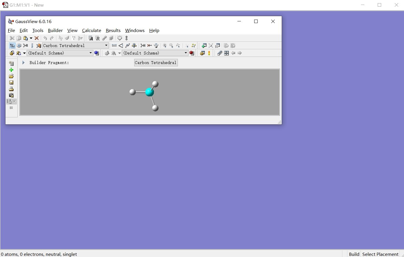
The GaussView used in this tutorial is the Windows version, while the interface for GaussView on Linux remains basically consistent. After opening GaussView, the interface appears as shown below.
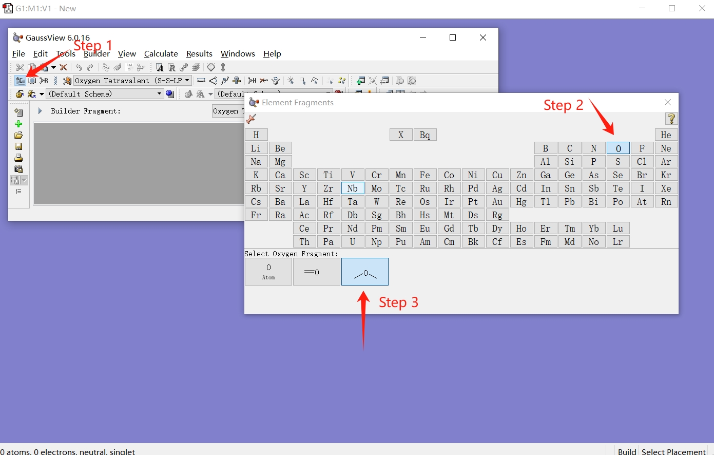
Follow the steps illustrated in the figure below to select the oxygen atom with automatically completed hydrogen atoms and click on the canvas to draw a water molecule.
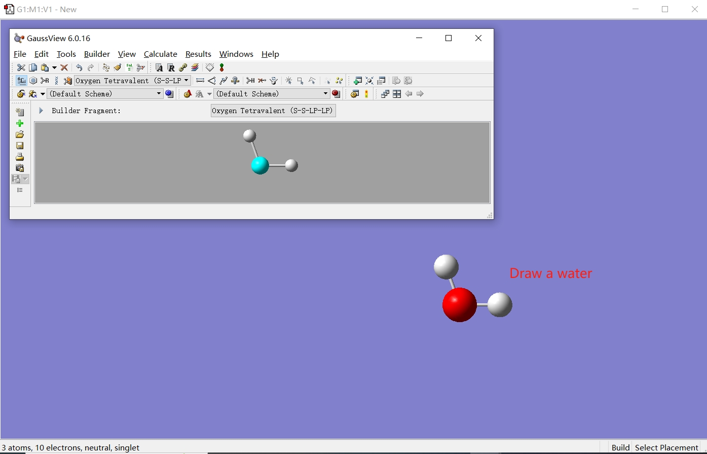
Then save the file as water1.pdb. At this point, we have obtained a PDB file containing a single water molecule.

Here is an example for water1.pdb:
REMARK   1 File created by GaussView 6.0.16
HETATM    1  O           0       0.061  -0.678   0.000                       O
HETATM    2  H           0       1.021  -0.678   0.000                       H
HETATM    3  H           0      -0.260   0.227   0.000                       H
END
CONECT    1    2    3
CONECT    2    1
CONECT    3    1
The third (atom name) and fourth (residue name) columns should be changed manually to:
REMARK   1 File created by GaussView 6.0.16
HETATM    1  O   WAT     0       0.061  -0.678   0.000                       O
HETATM    2  H1  WAT     0       1.021  -0.678   0.000                       H
HETATM    3  H2  WAT     0      -0.260   0.227   0.000                       H
END
CONECT    1    2    3
CONECT    2    1
CONECT    3    1
Note: The position of each column is strictly defined in PDB files. For example, the residue name must start from the 18th character. For detailed information, please refer to: Introduction to Protein Data Bank Format
Next, we use tleap to convert water1new.pdb into an AMBER-readable format. Ensure the pdb file and script file Reconstruct.leaprc are in the same dirctory. The specific command and script file are as follows:
tleap -f Reconstruct.leaprcwater=loadpdb water1new.pdb
savepdb water water1re.pdbThe reconstructed PDB file containing a single water molecule is shown below:
ATOM      1  O   WAT     1       0.061  -0.678   0.000  1.00  0.00
ATOM      2  H1  WAT     1       1.021  -0.678   0.000  1.00  0.00
ATOM      3  H2  WAT     1      -0.260   0.227   0.000  1.00  0.00
TER
END
At this stage, we can use packmol to generate a PDB file containing 216 water molecules using the following command and script file packmol.inp.
packmol < packmol.inptolerance 2.0
output water216.pdb
filetype pdb
structure water1re.pdb
number 216
inside cube 0. 0. 0. 19.
end structureFor details on the meaning of each line in the script file, please refer to: Section 2.3 of Tutorial for LSCIVR or Packmol userguide
Finally, tleap is used to generate the inpcrd and prmtop files for further simulations. The following command and script file qspcfw.leaprc are used.
tleap -f qspcfw.leaprcsource leaprc.protein.ff14SB
loadOff solvents.lib # load atom names library and residue name library for solvent
WAT = SPG # set residue name WAT equal to SPG
loadAmberParams frcmod.qspcfw # load parameters for q-SPC/fw model
set default FlexibleWater on # using flexible water model
water = loadpdb "water216.pdb" # load coordinate file in pdb format
setBox water centers 0.0 # set box centers at (0.0,0.0,0.0), and generate box automatically
saveamberparm water wat216.prmtop wat216.inpcrd # save topology file and coordinate file
quitMinimizing the energy of the system
The coordinate files generated by packmol often have high strain and should always undergo configuration optimization using AMBER's energy minimization function to prevent molecular dynamics simulation crashes. The input file for energy minimization is shown below:
minimization
 &cntrl
 imin   = 1,
 maxcyc = 50000,
 ncyc   = 25000,
 ntb    = 1,
 cut    = 7.0
  /
Run the minimization with sander:
sander -O -i min.in -p wat216.prmtop -c wat216.inpcrd -o min.out -r min.rstThe details of paramters in the input file can be found in Section 2.4 of Tutorial for LSCIVR or AMBER manual.
Equilibrating and Sampling the system using classical dynamics (NPT)
In this section, we will calculate the isobaric heat capacity, isothermal compressibility and thermal expansion coefficient of liquid water at 298 K and 1 atm using classical molecular dynamics. The minimized configuration containing 216 water molecules min.rst generated in the previous step will serve as the initial configuration. The input files (‘npt1.in’ and ‘npt2.in’) are as follows:
NPT simulation of liquid water
&cntrl
imin = 0,
irest = 0, ntx = 1,
ntb = 2, cut = 7.0,
ntp = 1, taup = 2.0, pres0 = 1.013, barostat = 1, baro_stochastic = 1,
tempi = 298.15, temp0 = 298.15,
ischeme = 1, ithermostat = 1, therm_par = 5.0, ig = -1,
nstlim = 500000, dt = 0.002,
ntpr = 1000, ntwx = 1000, ntwr = 1000,
/
&ewald
skinnb = 2.0
 /
NPT simulation of liquid water
&cntrl
imin = 0,
irest = 1, ntx = 5,
ntb = 2, cut = 7.0,
ntp = 1, taup = 2.0, pres0 = 1.013, barostat = 1, baro_stochastic = 1,
tempi = 298.15, temp0 = 298.15,
ischeme = 1, ithermostat = 1, therm_par = 5.0, ig = -1,
nstlim = 5000000, dt = 0.002,
ntpr = 50, ntwx = 1000, ntwr = 1000,
/
&ewald
skinnb = 2.0
 /
The details of paramters in the input file can be found in Section 3.1 of Tutorial for LSCIVR or AMBER manual. The parameters for the "middle" scheme are listed in Input parameters.
Typically, we need to run multiple trajectories (more than 20) to obtain sufficiently converged results. Here, we use a bash script run.sh to circularly generate trajectories, with each sampled trajectory employing a distinct initial configuration. Each trajectory will be generated in a folder numbered correspondingly.
#!/bin/bash
cp min.rst start.rst.1
for i in {1..20}
do
  mkdir $i
  cp start.rst.$i $i/;
  cd $i;
  pmemd -O -i npt1.in -p wat216.prmtop -c start1.rst  -o equi.out -r equi.rst.$i -x equi.mdcrd;
  pmemd -O -i npt2.in -p wat216.prmtop -c equi.rst.$i  -o sample.out -r end.rst.$i -x equi.mdcrd;
  cp equi.rst.$i ../start.rst.$((i+1));
  cd ../;
done
Analysis
We can analyze the output files using the process_mdout.perl script included in the AMBER package to generate data files containing sampled quantities (e.g., volume, energy). For the calculation of different thermodynamic properties, a python script NPT_static.py is provided. The calculation method can be found in Ref [JCTC].
We also provide a loop analysis script to analyze each trajectory. The properties of each trajectory will be printed into TXT files within their respective folders. For example, the isobaric heat capacity analysis result is saved as Cp.txt.
#!/bin/bash
for i in {1..20}
do
  cp NPT_static.py $i/;
  cd $i;
  process_mdout.perl sample.out
  python NPT_static.py
  cd ../;
done
Test cases
Molecular dynamics (for classical statistics)
(a) MD input using the Langevin thermostat with the “LFMiddle” scheme for liquid water.
Test: $AMBERHOME/test/middle-scheme/MD_Unconstr_Langevin_water
MD: NVT simulation of liquid water
&cntrl
ipimd = 0, nstlim = 10        ! MD for 10 steps
ntx = 1, irest = 0            ! read coordinates
temp0 = 300, tempi = 300      ! temperature: target and initial
dt = 0.001                    ! time step in ps
cut = 7.0                     ! non-bond cut off
ischeme = 1                   !! leapfrog middle scheme
ithermostat = 1               !! Langevin thermostat
therm_par = 5.0               !! thermostat parameter in 1/ps
ig = 1000                     ! random seed
ntc = 1, ntf = 1              ! no constraints
ntpr = 1, ntwr = 5, ntwx = 5  ! output settings
/
One can run either a serial job (using sander ):
$ sander -O -i md_LGV.in -p qspcfw216.top -c nvt.rst -o md_LGV.out \
  -r lgv.rst -info lgv.info
or a parallel job (using sander.MPI ):
$ mpirun -np 4 sander.MPI -O -i md_LGV.in -p qspcfw216.top -c nvt.rst \
  -o md_LGV.out -r lgv.rst -info lgv.info
(b) MD input using Langevin dynamics with the “LFMiddle” scheme for the liquid water. Lengths of the bonds having hydrogen atoms are constrained.
Test: $AMBERHOME/test/middle-scheme/MD_Constr_Langevin_water
MD: NVT simulation of liquid water
&cntrl
ipimd = 0, nstlim = 10        ! MD for 10 steps
ntx = 1, irest = 0            ! read coordinates
temp0 = 300, tempi = 300      ! temperature: target and initial
dt = 0.004                    ! time step in ps
cut = 7.0                     ! non-bond cut off
ischeme = 1,                  !! leapfrog middle scheme
ithermostat = 1,              !! Langevin thermostat, random seed is default value
therm_par = 5.0               !! thermostat parameter, in 1/ps
ntc = 2, ntf = 2              ! constrain lengths of the bonds having hydrogen atoms
ntpr = 1, ntwr = 5, ntwx = 5  ! output settings
/
Run either a serial way (using sander ):
$ sander -O -i md_LGV.in -p qspcfw216.top -c nvt.rst -o md_LGV.out \
  -r lgv.rst -info lgv.info
or a parallel job (using sander.MPI ):
$ mpirun -np 4 sander.MPI -O -i md_LGV.in -p qspcfw216.top -c nvt.rst \
  -o md_LGV.out -r lgv.rst -info lgv.info
(c) MD input using Langevin dynamics and stochastic cell rescaling barostat with the “LFMiddle” scheme for the liquid water in the isothermal-isobaric (NPT) ensemble. Lengths of the bonds having hydrogen atoms are constrained.
Test: $AMBERHOME/test/middle-scheme/MD_NPT_Constr_Langevin_water
MD: NPT simulation of liquid water
&cntrl
ntx = 1, irest = 0                ! read coordinates
ntc=2, ntf=2, tol=0.0000001,      ! constrain lengths of bonds
                                  ! having hydrogen atoms
ntb = 2,                          ! constant pressure simulation
ntp = 1,                          ! md with isotropic position scaling
barostat = 1,                     ! using Berendsen barostat
baro_stochastic = 1,              !! Adds a stochastic term to the barostat
taup = 2.0,                       ! pressure relaxation time, in ps
pres0 = 1.013,                    ! reference external pressure, in bar
nstlim=10,                        ! MD for 10 steps
ntpr=1, ntwr=10000,               ! output settings
dt=0.004,                         ! timestep in ps
ig=71277,                         ! random seed
cut = 7.0,                        ! non-bond cut off
temp0 = 300, tempi = 300,         ! temperature: target and initial
ischeme = 1,                      !! Leapfrog middle scheme
ithermostat = 1,                  !! Langevin thermostat
therm_par = 5.0,                  !! thermostat parameter in ps^-1
/
/
Run either a serial way (using sander ):
$ sander -O -i md_LGV_SCR.in -p qspcfw216.top -c npt.rst -o md_LGV_SCR.out \
  -r lgv_scr.rst -info lgv_scr.info
or a parallel job (using sander.MPI ):
$ mpirun -np 4 sander.MPI -O -i md_LGV_SCR.in -p qspcfw216.top -c npt.rst \
  -o md_LGV_SCR.out -r lgv_scr.rst -info lgv_scr.info
Path integral molecular dynamics (for quantum statistics)
(d) PRIMPIMD input using the Andersen thermostat with the “LFMiddle” scheme for the liquid water. Lengths of the bonds having hydrogen atoms are constrained.
Test: $AMBERHOME/test/middle-scheme/PIMD_Constr_Andersen_water
PRIMPIMD: NVT simulation of liquid water
&cntrl
ipimd = 1, nstlim = 10   ! PRIMPIMD for 10 steps
ntx = 5, irest = 0       ! read coordinates
temp0 = 300, tempi = 300 ! target temperature and initial temperature
dt = 0.002               ! time step in ps
cut = 7.0                ! non-bond cut-off
ischeme = 1,             !! leapfrog middle scheme
ithermostat = 2,         !! Andersen thermostat
therm_par = 8.0          !! thermostat parameter, in 1/ps
ig = 777                 ! random seed
ntc = 2,ntf = 2          ! constrain lengths of the bonds having hydrogen atoms
ntpr=1, ntwr=5, ntwx=5   ! output settings
/
(e) PRIMPIMD input using Langevin dynamics with the “LFMiddle” scheme for the liquid water. No constraints are applied.
Test: $AMBERHOME/test/middle-scheme/PIMD_Langevin_water
PRIMPIMD: NVT simulation of liquid water
&cntrl
ipimd = 1,nstlim = 10   ! PRIMPIMD for 10 steps
ntx = 5,irest = 0       ! read coordinates,
                        ! and run as a new simulation.
temp0 = 300,tempi = 300 ! target and initial temperature
dt = 0.001              ! time step, in ps
cut = 7.0               ! non-bond cut off
ischeme = 1,            !! leapfrog middle scheme
ithermostat = 1,        !! Langevin thermostat
therm_par = 5.0         !! thermostat parameter, in 1/ps
ntc = 1                 ! no constraints, default
ntpr=1, ntwr=5, ntwx=5  ! output settings
/
(f) PRIMPIMD input using Langevin dynamics with the “LFMiddle” scheme for the liquid water. No constraints are applied.
Test: $AMBERHOME/test/middle-scheme/PIMD_NPT_Langevin_water
PRIMPIMD: NVT simulation of liquid water
&cntrl
ipimd = 2, nstlim = 10   ! NMPIMD for 10 steps
ntx = 5, irest = 0       ! read coordinates
                         ! and run as a new simulation.
temp0 = 300, tempi = 300 ! target and initial temperature
dt = 0.001               ! time step in ps
cut = 7.0                ! non-bond cut off
ischeme = 1,             !! Leapfrog middle scheme
ithermostat = 1,         !! Langevin thermostat
therm_par = 5.0          !! thermostat parameter, in 1/ps
                         !! (friction coefficient for Langevin thermostat)
therm_vol = 2.0          !! barostat parameter, in 1/ps
                         !! (friction coefficient for MTTK-Langevin barostat)
ntb = 2,                 ! constant pressure simulation
ntp = 1,                 ! md with isotropic position scaling
barostat = 1,            ! using MTTK-Langevin equation
                         ! only work as MTTK when using NMPIMD
taup = 2.0,              ! pressure relaxation time, in ps
pres0 = 1.013,           ! reference external pressure, in bar
ntc = 1                  ! no constraints, default
ntpr=1, ntwr=5, ntwx=5   ! output settings
/
/
When one runs PIMD in AMBER, a groupfile is needed. The groupfile gf_pimd may look like:
-O -i pimd.in -p qspcfw216.top -c nvt1.rst -o bead1.out -r bead1.rst
 -x bead1.mdcrd -inf bead1.mdinfo
-O -i pimd.in -p qspcfw216.top -c nvt2.rst -o bead2.out -r bead2.rst
 -x bead2.mdcrd -inf bead2.mdinfo
-O -i pimd.in -p qspcfw216.top -c nvt3.rst -o bead3.out -r bead3.rst
 -x bead3.mdcrd -inf bead3.mdinfo
-O -i pimd.in -p qspcfw216.top -c nvt4.rst -o bead4.out -r bead4.rst
 -x bead4.mdcrd -inf bead4.mdinfo
Note that each line starts with -O and ends with -inf <info> . The groupfile above contains 4 lines, which means 4 path integral beads are used.
sander.MPI is executed via the following command:
$ mpirun -np 8 sander.MPI -ng 4 -groupfile gf_pimdThe number of processes (8) that is specified by -np is a multiple of the number of groups (4). In this case 2 CPU processes are used on each path integral bead.
QM/MM molecular dynamics
(g) QM/MM MD input using the Langevin thermostat with the “LFMiddle” scheme for the alanine dipeptide solved in methol box. Lengths of the bonds having hydrogen atoms are constrained for the MM part, while no constraints are applied to the QM part.
Test: $AMBERHOME/test/middle-scheme/QMMM_Constr_ALA_Methol
constrained MD NVT: Alanine dipeptide in meoh (explicit solvent).
&cntrl
ipimd = 0, nstlim = 10,   ! MD for 10 steps
irest = 0, ntx = 1,       ! read coordinates
temp0 = 300               ! target temperature
tempi = 300               ! initial temperature
dt = 0.002,               ! time step, in ps
cut = 8,                  ! non-bond cut off
ig = 6666,                ! random seed for reproducing results
ischeme = 1,              !! leapfrog middle scheme
ithermostat = 1           !! Langevin thermostat
therm_par = 5.0,          !! thermostat parameter, in 1/ps
ntc=2,ntf=2               ! constrain lengths of bonds having hydrogen atoms
 atoms
ntpr=1, ntwr=1, ntwx=1    ! output settings
ifqnt=1                   ! switch on QM/MM coupled potential
/
&qmmm qmmask=':ACE,ALA,NME', ! residues treated using QM
qmcharge=0,            ! charge on QM region is 0
qmshake=0,             ! no SHAKE for QM region
qm_theory='PM3',       ! use the PM3 semi-empirical Hamiltonian
qmcut=8.0              ! use 8 angstrom cut off for QM region
/
One can run either a serial job (using sander ):
$ sander -O -i qmmm.in -p ala.top -c ala.crd -o qmmm.out -r qmmm.rst \
  -x qmmm.crd -info qmmm.info
or a parallel job (using sander.MPI ):
$ mpirun -np 4 sander.MPI -O -i qmmm.in -p ala.top -c ala.crd \
  -o qmmm.out -r qmmm.rst -x qmmm.crd -info qmmm.info
Replica exchange molecular dynamics
(h) REMD input using the Langevin thermostat with the “LFMiddle” scheme for the ACE-ALA-ALA-ALA-NME in vacuum.Lengths of the bonds having hydrogen atoms are constrained.
Test: $AMBERHOME/test/middle-scheme/REMD_Constr_ALA
Below is the input file for one of the replicas. The target temperatures are 300, 325, 350, and 400K for the 4 replicas, respectively.
REMD test with 4 replicas
&cntrl
imin = 0, nstlim = 100,     ! MD for 100 steps
irest=1,ntx = 5,            ! read coordinates and velocities
tempi = 0.0, temp0 = 300.0, ! initial and target temperature
ischeme= 1,                 !! leapfrog middle scheme
ithermostat = 1,            !! Langevin thermostat
therm_par = 1.0,            !! thermostat parameter,in 1/ps
dt = 0.002,                 ! time step, in ps
ig=6666,                    ! random seed
ntc = 2, ntf = 2,           ! constrain lengths of the bonds having hydrogen atoms
ntwx = 50, ntwr =50, ntpr = 50,  ! output setting
ntb=0,                      ! no periodicity
cut = 99.0,                 ! non bond cut off
numexchg=5,                 ! exchange frequency
&end
When one runs REMD in AMBER, a groupfile is needed. The groupfile groupfile may look like:
-O -rem 1 -remlog rem.log -i rem.in.000 -p ala3.top -c mdrestrt -o rem.out.000
 -r rem.r.000 -inf reminfo.000
-O -rem 1 -remlog rem.log -i rem.in.001 -p ala3.top -c mdrestrt -o rem.out.001
 -r rem.r.001 -inf reminfo.001
-O -rem 1 -remlog rem.log -i rem.in.002 -p ala3.top -c mdrestrt -o rem.out.002
 -r rem.r.002 -inf reminfo.002
-O -rem 1 -remlog rem.log -i rem.in.003 -p ala3.top -c mdrestrt -o rem.out.003
 -r rem.r.003 -inf reminfo.003
Note that each line starts with -O and ends with -inf <info> . The groupfile has 4 lines, which means 4 replicas are employed in REMD. sander.MPI is executed via the following command:
$ mpirun -np 4 sander.MPI -ng 4 -groupfile groupfileThe number of processes (4) that is specified by -np can be replaced by any multiple of the number of replicas used in REMD (4 in this case).
Pmemd examples for CPU and GPU
(i) Pmemd input for liquid water with 4096 water molecules in a cell
Test: $AMBRHOME/test/middle-scheme/4096wat
MD: NVT simulation of liquid water
&cntrl
ntx = 5, irest = 1, ! read coordinates
ntc = 2, ntf = 2, ! constrain lengths of bonds
tol = 0.0000001, ! having hydrogen atoms
nstlim = 10, ! MD for 10 steps
ntpr = 1, ntwr = 10000 ! output settings
dt = 0.001, ! timestep in ps
ig = 71277, ! random seed
cut = 7.0, ! non-bond cut off
ischeme = 1, !! Leapfrog middle scheme
ithermostat = 1, !! Langevin thermostat
therm_par = 5.0, !! thermostat parameter
midpoint = 1 ! use midpoint method, only for pmemd.MPI;
! remove this flag otherwise
/
&end
(j) Pmemd input for liquid water with 4096 water molecules in the isothermal-isobaric (NPT) in a cell
Test: $AMBRHOME/test/middle-scheme/4096wat
MD: NPT simulation of liquid water
&cntrl
ntx = 5, irest = 1,         ! read coordinates
ntc = 2, ntf = 2,           ! constrain lengths of bonds
tol = 0.0000001,            ! having hydrogen atoms
ntb = 2,                    ! constant pressure simulation
ntp = 1,                    ! md with isotropic position scaling
barostat = 1,               ! using Berendsen barostat
baro_stochastic = 1,        !! Adds a stochastic term to the barostat
taup = 2.0,                 ! pressure relaxation time, in ps
pres0 = 1.013,              ! reference external pressure, in bar
nstlim = 10,                ! MD for 10 steps
ntpr = 1, ntwr = 10000      ! output settings
dt = 0.001,                 ! timestep in ps
ig = 71277,                 ! random seed
cut = 7.0,                  ! non-bond cut off
ischeme = 1,                !! Leapfrog middle scheme
ithermostat = 1,            !! Langevin thermostat
therm_par = 5.0,            !! thermostat parameter, in 1/ps
/
&end
(k) Pmemd input for DNA A7 −T7 duplex solvated in a cell with 3351 water molecules and 12 sodium ions as counter-ions
Test: $AMBERHOME/test/middle-scheme/DNA7
MD: NVT simulation of DNA duplex
&cntrl
ntx = 5, irest = 1, ! read coordinates
ntc = 2, ntf = 2, ! constrain lengths of bonds
tol = 0.0000001, ! having hydrogen atoms
nstlim = 10, ! MD for 10 steps
ntpr = 1, ntwr = 10000 ! output settings
dt = 0.001, ! timestep in ps
ig = 71277, ! random seed
cut = 9.0, ! non-bond cut off
ischeme = 1, !! Leapfrog middle scheme
ithermostat = 1, !! Langevin thermostat
therm_par = 5.0, !! thermostat parameter
midpoint = 1 ! use midpoint method, only for pmemd.MPI;
! remove this flag otherwise
/
(l) Pmemd input for Ethaline Deep Eutectic Solvent(512 choline chloride and 1024 ethylene glycol molecules)
Test: $AMBERHOME/test/middle-scheme/ETH
MD: NVT simulation of Ethaline Deep Eutectic Solvent
&cntrl
ntx = 5, irest = 1, ! read coordinates
ntc = 2, ntf = 2, ! constrain lengths of bonds
tol = 0.0000001, ! having hydrogen atoms
nstlim = 10, ! MD for 10 steps
ntpr = 1, ntwr = 10000 ! output settings
dt = 0.001, ! timestep in ps
ig = 71277, ! random seed
cut = 10.0, ! non-bond cut off
ischeme = 1, !! Leapfrog middle scheme
ithermostat = 1, !! Langevin thermostat
therm_par = 5.0, !! thermostat parameter
midpoint = 1 ! use midpoint method, only for pmemd.MPI;
! remove this flag otherwise
/
&end
(m) Pmemd input for 1:6 methanol-zinc chloride solution (290 zinc chloride and 1740 methanol molecules)
Test: $AMBERHOME/test/middle-scheme/MeOHZnCl2
MD: NPT simulation of 1:6 methanol-zinc chloride solution
&cntrl
ntx=5, irest=1,                   ! read coordinates
ntb = 2,                          ! constant pressure simulation
ntp = 1,                          ! md with isotropic position scaling
barostat = 1,                     ! using Berendsen barostat
baro_stochastic = 1,              !! Adds a stochastic term to the barostat
taup = 2.0,                       ! pressure relaxation time, in ps
pres0 = 1.013,                    ! reference external pressure, in bar
nstlim=10,                        ! MD for 10 steps
ntpr=1, ntwr=10000,               ! output settings
dt=0.002,                         ! timestep in ps
ig=71277,                         ! random seed
cut = 7.0,                        ! non-bond cut off
temp0 = 300, tempi = 300,         ! temerature settings
ischeme = 1,                      !! Leapfrog middle scheme
ithermostat = 1,                  !! Langevin thermostat
therm_par = 5.0,                  !! thermostat parameter in ps^-1
/
&end
All those pmemd examples can be executed in a serial job(using sander or pmemd):
$ sander -O -i mdin -o mdout -p prmtop -c inpcrd -r restrtor
$ pmemd -O -i mdin -o mdout -p prmtop -c inpcrd -r restrtor a parallel job(using sander.MPI or pmemd.MPI):
$ sander.MPI -O -i mdin -o mdout -p prmtop -c inpcrd -r restrtor
$ pmemd.MPI -O -i mdin -o mdout -p prmtop -c inpcrd -r restrtor a GPU-accelerated job(using pmemd.cuda):
$ pmemd.cuda_DPFP -O -i mdin -o mdout -p prmtop -c inpcrd -r restrt
$ pmemd.cuda_SPFP -O -i mdin -o mdout -p prmtop -c inpcrd -r restrt
References
[1] Zhang, Z.; Liu, X.; Chen, Z.; Zheng, H.; Yan, K.; Liu*, J. A unified thermostat scheme for efficient configurational sampling for classical/quantum canonical ensembles via molecular dynamics. The Journal of Chemical Physics 2017, 147 (3), 034109 [DOI: 10.1063/1.4991621]. [pdf version]
[2] Liu*, J.; Li, D.; Liu, X. A simple and accurate algorithm for path integral molecular dynamics with the Langevin thermostat. The Journal of Chemical Physics 2016, 145 (2), 024103 [DOI: 10.1063/1.4954990].[pdf version]
[3] Li, D.; Han, X.; Chai, Y.; Wang, C.; Zhang, Z.; Chen, Z.; Liu*, J.; Shao*, J. Stationary state distribution and efficiency analysis of the Langevin equation via real or virtual dynamics. The Journal of Chemical Physics 2017, 147 (18), 184104 [DOI: 10.1063/1.4996204]. [pdf version]
[4] Li, D.; Chen, Z.; Zhang, Z.; Liu*, J. Understanding Molecular Dynamics with Stochastic Processes via Real or Virtual Dynamics. Chinese Journal of Chemical Physics 2017, 30 (6), 735–760 [DOI: 10.1063/1674-0068/30/cjcp1711223][The paper is available from the official CJCP website]. [pdf version]
[5] Zhang, Z.; Yan, K.; Liu, X.; Liu*, J. A Leap-Frog Algorithm-Based Efficient Unified Thermostat Scheme for Molecular Dynamics. Chinese Science Bulletin 2018, 63 (33), 3467–3483 [DOI: 10.1360/N972018-00908]. [pdf version]
[6] Leimkuhler, B.; Matthews, C. Rational Construction of Stochastic Numerical Methods for Molecular Sampling. Applied Mathematics Research eXpress 2013, 2013 (1), 34–56 [DOI: 10.1093/amrx/abs010].
[7] Grønbech-Jensen, N.; Farago, O. A simple and effective Verlet-type algorithm for simulating Langevin dynamics. Molecular Physics 2013, 111 (8), 983–991 [DOI: 10.1080/00268976.2012.760055].
[8] Liu, X.; Liu*, J. Critical role of quantum dynamical effects in the Raman spectroscopy of liquid water. Molecular Physics 2018, 116 (7-8), 755–779 [DOI: 10.1080/00268976.2018.1434907]. [pdf version]
[9] Ryckaert, J.-P.; Ciccotti, G.; Berendsen, H. J. Numerical Integration of the Cartesian Equations of Motion of a System with Constraints: Molecular Dynamics of N-Alkanes. Journal of Computational Physics 1977, 23 (3), 327–341 [DOI: 10.1016/0021-9991(77)90098-5].
[10] Andersen, H. C. RATTLE: A "velocity" version of the shake algorithm for molecular dynamics calculations. Journal of Computational Physics 1983, 52 (1), 24–34 [DOI: 10.1016/0021-9991(83)90014-1].
[11] Miyamoto, S.; Kollman, P. A. Settle: An analytical version of the SHAKE and RATTLE algorithm for rigid water models. Journal of Computational Chemistry 1992, 13 (8), 952–962 [DOI: 10.1002/jcc.540130805].
[12] Zhang, Z.; Liu X.; Yan, K.; Tuckerman, M.; Liu*, J. A unified efficient thermostat scheme for the canonical ensemble with holonomic or isokinetic constraints via molecular dynamics. Journal of Physical Chemistry A 2019, 123 (28), 6056-6079 [DOI: 10.1021/acs.jpca.9b02771]. (Invited contribution to "Young Scientist Virtual Special Issue"; Highlighted in JPC Virtual Issue on New Tools and Methods )
[13] Andersen, H. C. Molecular dynamics simulations at constant pressure and/or temperature. The Journal of Chemical Physics 1980, 72 (4), 2384–2393 [DOI: 10.1063/1.439486].
[14] Sun, Z.; Kalhor, P.; Xu, Y.; Liu*, J., Extensive Numerical Tests of Leapfrog Integrator in Middle Thermostat Scheme in Molecular Simulations. Chinese Journal of Chemical Physics 2021, 34. [DOI: 10.1063/1674-0068/cjcp2111242].
[15] Rogge, S. M. J.; Vanduyfhuys, L.; Ghysels, A.; Waroquier, M.; Verstraelen, T.; Maurin, G.; Van Speybroeck*, V., A Comparison of Barostats for the Mechanical Characterization of Metal–Organic Frameworks. The Journal of Chemical Theory and Computation 2015, 11, 5583-5597. [DOI: 10.1021/acs.jctc.5b00748].
[16] Bernetti, M.; Bussi*, G., Pressure Control Using Stochastic Cell Rescaling. The Journal of Chemical Physics 2020, 153, 114107. [DOI: 10.1063/5.0020514].
[17] Martyna, G. J.; Hughes, A.; Tuckerman*, M. E., Molecular Dynamics Algorithms for Path Integrals at Constant Pressure. The Journal of Chemical Physics 1999, 110, 3275-3290. [DOI: 10.1063/1.478193].